Where β   0. In section 2, we discuss some basic definitions on fuzzy set theory with properties and theorems. In section 4, we anticipated an algorithm about the LFFPP. In next section, we discuss a simple numerical example on LFFPP by simplex method. In last section, we provided the concluding remarks

 

2. PRELIMINARIES

This section contains basic preliminary definitions and its some properties, which will be used in a sequel.

 

2.1. DEFINITIONS

1)    Fuzzy set: Let X be a general set and x be a member of X, then fuzzy set   on X is denoted by a membership value µ_ () (x), which identifies the function maps from every element to the interval Bitran and Novaes (1972) and it can be defined as

 

 

               Where

        

2)    α − cut: Let be a fuzzy set on X and α be a real number between Bitran and Novaes (1972), then cut of   is determined by

  
                                                                      

 

3)    Strong α − cut: Let  be a fuzzy set on X and α be a real number between [0, 1], then strong α − cut of fuzzy set    is defined as

 

 

4)    Support of a fuzzy set: Consider X be a crisp set and   be a fuzzy set associate on X. Then support of    is described by

 

                        

                  

5)    Normal Fuzzy set: Let X be a universal set  be a fuzzy section X. Then normal of fuzzy set is termed as

 

 

 

 

6)    Convex of fuzzy set:  consider X be a crisp set. A fuzzy subset  on X is convex if and only if

 

 and

        

7)    Fuzzy Number: A fuzzy set   on X is a fuzzy number if and only if it is normal and convex in X

 

8)    Triangular fuzzy number: The triangular fuzzy number of fuzzy sets   is a triplet product [l, m, n] and its value of it corresponding the membership function is defined by

                         

                                                                                                           

 

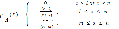
Where l and n are representing the lower and the upper boundaries respectively, with membership degree is 0 and m is the centre with membership degree is 1

 

9)    Arithmetic Operations: Let        = (l_1, m_1, n1) and      = (l_2, m_2, n_2) be two triangular fuzzy numbers, then

 

·        Addition

 

·        Substraction

                                            

                                       = ()+()+()

 

·        Multiplication

 

 

 

 

 

·        Scalar Multiplication

 

                      ,) = (k)   if k

 

                      ,) = (k)   if k

 

·        Division

10)    Ranking Function: The ranking function “R” is a mapping from each fuzzy number into the set of real line and it is defined by

 

                                          

 

Where the F(R) consists of triangular fuzzy numbers.

If     be the triangular fuzzy number, then the corresponding ranking function of     is given by 

 

                                            

 

11)    Efficient point: A point x0 is called to be an efficient point if there does not exist other feasible point x other than x0,

i.e

 

                                                                                                     

 

Theorem 1. Narayanamoorthy and Kalyani (2015) Suppose X_t is the set of efficient points for P_t, t = 1, 2, then X_t is a subset of the set of all efficient points X of P

 

Theorem 2. Hitchcock  (1941) Suppose  be an optimal solution of P₁ and   = {x_i ∈P} be an another optimal solution of P₂,then     is an optimal solution of P,

Where all elements of x₁, x₂. are in P₁ and P₂.

 

1)    Linear Fractional Fuzzy Programming Problem (LFFPP)

In this section, we expand the linear fractional problem into linear fractional fuzzy programming problem. The LFFPP can be considered as:

 

                                            

 

Subject to

 

                                                     Equation 1

 

Where p(x) and q(x) are continuous linear functions and   q(x) > 0, x now the set S is designated by

 

                                           

 

Where S is a bounded polyhedron and     is a fuzzy matrix of order. Now n×n the above equation may be represented as

 

 

                                 

 

                        

                         Equation 2

 

Then by using above theorem-2, we have the set of efficient points for p_t, t = 1, 2 is a subset of p.

 

3. ALGORITHM

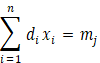
This section deals with a methodology for solving a linear fractional fuzzy trans- potation problem (LFFTP). The LFFTP can be considered as

 

 

 

 

 

 

                     Equation 3

 

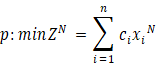
Where the objective function is of fractional type. This problem can be decom- posed into two linear fuzzy problem such as

 

Subject to

 

 

 

                                                                     Equation 4

 

                                                                                                                              

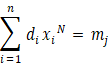
Subject to

                                                                                                                             

 

                                                                                                                             

 

                                                                                           Equation 5

 

Then by simplex method, we have to find the solution of two linear fuzzy problems. Thus, the solutions min z^N and min z^D are determined distinctly. Then by the above theorem, we have to obtain the optimal solution of P

 

4. NUMERICAL EXAMPLE

Here, we demonstrate a numerical example on linear fractional transportation problems under fuzzy values which are expressed by a triangular fuzzy number. Consider a LFFTP as:

 

                                                                         

 

           

 

         

 

                                                                          Equation 6

 

Where objective function is expressed in case of triangular fuzzy number and crisp values for case of supply and demands.

In computationally, this problem can be written as

 

                                           

 

Subject to

                    

 

                     

 

and

 

Subject to

                                                              

 

               

 

                  

 

                                                                                   Equation 7

 

The standard form of the linear problem P1 can be expressed as

 

                                                                      

Subject to

 

 

 

 

Where s₁ and s₂ are basic slack variables.

Now to solve

LFTP ′P₁′ with the help of simplex method. The initial simplex table is given as

Table 1
		cj	(-8,2,5)	(10, -2, -6)	(0,0,0)	(0,0,0)3	Min
CB	YB	XB	X1	X2	S1	S2
(0,0,0)	S1	6	3	2	1	0	2
(0,0,0)	S2	10	4	5	0	1	2.5
	Zj	0	0	0	0	0
	Zj-Cj		(-5, -2, -8)	(6,2, -10)	0	0
	R		-0.84	0.67	0	0

 

In this above table, we have one zj cj   value is non-positive. So, the feasible optimal solution has been not reached. The   non -basic variable s1 will go away the basis cell and the basic variable x1 come into the basis cell.

Table 2
		cj	(-8,2,5)	(10, -2,6)	(0,0,0)	(0,0,0)3
CB	YB	XB	X1	X2	S1	S2
(-8,2,5)	X1	2	1	2/3	1/3	0
0	S2	2	0	7/3	-4/3	1
	Zj	(-16,4,10)	(-8,2,5)	(-16/3,4/3,10/3)	(-8/3,2/3,5/3	(0,0,0)
	Zj-Cj		0	(-46/3,10/3,28/3)	(-8/3,2/3,5/3)	0
	R		0	1.23	0.28	0

 

Now using the procedure of simplex method, we get the following table.

   This table shows that all zj - cj ≥ 0 so optimal solution to the LFTP is obtained 

Thus, the solution is

 

                 x₁ = 2, x₂ = 0, max z^N = (−16, 4, 10)

i.e.

               x₁ = 2, x₂ = 0, min z^N = (−10, −4, 16).               Equation 8

 

Similarly consider the standard form of the linear problem P2 can be expressed as

            P₂: max z^D = ((6, −4, −4) x₁ + (−4, 4, 4) x₂)

Subject to

                  3x₁ + 2x₂ + s₁ = 6

 

                  4x₁ + 5x₂ + s₂ = 10

 

                                                                   x₁, x₂, s₁, s₂ ≥ 0,                                     Equation 9

 

Where s₁ and s₂ are slack variables. Now to solve the LFTP “p₂” and simplex method. The primary datas are given below.

Table 3
		Cj	(-6,4,4)	(4, -4, -4)	(0,0,0)	(0,0,0)3	Min
CB	YB	XB	X1	X2	S1	S2
(0,0,0)	S1	6	3	2	1	0	2
(0,0,0)	S2	10	4	5	0	1	2.5
	Zj	0	0	0	0	0
	Zj-Cj		(-4, -4,6)	(4,4, -4)	0	0
	R		-2.34	2.67	0	0

 

From the above table, we get one    value is negative. So, the optimal feasible solution is not satisfied. Thus, the non-basic variable s1 will leave the basis and the basic variable x1 enter the basis.

Now by using the procedure of simplex method, we have the following table.

Table 4
		cj	(-6,4,4)	(4, -4, -4)	(0,0,0)	(0,0,0)3
CB	YB	XB	X1	X2	S1	S2
(-6,4,4)	X1	2	1	2/3	1/3	0
0	S2	2	0	7/3	-4/3	1
	Zj	(-12,8,8)	(-6,4,4)	(-4,8/3,8/3)	(-2,4/3,4/3)	(0,0,0)
	Zj-Cj		0	(-8,20/3,20/3)	(-2,4/3,4/3)	0
	R		0	4.23	0.78	0

 

This table shows that all. , it implies that the optimality condition is satisfied so,

 

                         = (−12, 8, 8)

i.e.

 

                                 Equation 10

 

So, the required optimum value is

 

                 Equation 11

 

 

5. CONCLUSION

In this research article, we anticipated a methodology for finding a solution of linear fractional fuzzy transportation problem, where objective functions are expressed by tri-angular fuzzy number. This proposed method i.e., simplex method is one of the exclusive techniques for calculating the optimal solution of any transportation problem. This additionally be prolonged into fractional quadratic problems.

 

ACKNOWLEDGEMENT

This research is supported and funded by C.V Raman Global University, Bhubaneswar, Odisha, India.

 

REFERENCES

Bitran, G. R. and Novaes, A. G. (1972) : Linear programming with a fractional objective function, Operations Research, 21, (1), 22-29. https://doi.org/10.1287/opre.21.1.22

Chandra, S. (1968) : Decomposition principle for linear fractional functional programs, Revue Francaise d'Informatique et de Recherche Operationnelle, 10, 65-71,  https://doi.org/10.1051/m2an/196802R200651

Charnes, A. and Cooper, W. W. (1973) : An explicit general solution in linear fractional program- ming, Naval Research Logistics, 20,(3), 449-467, https://doi.org/10.1002/nav.3800200308

Hitchcock, F. L. (1941) : The distribution of a product from several sources to numerous localities, Journal of Mathematics and Physics, 20, 224-230, https://doi.org/10.1002/sapm1941201224

Narayanamoorthy, S. and Kalyani, S. (2015) : The Intelligence of Dual Simplex Method to Solve Linear Fractional Fuzzy Transportation Problem, Computational Intelligence and Neuroscience, https://doi.org/10.1155/2015/103618

Pandian, P. and Jayalakshmi, M. (2013) : On solving linear fractional programming problems, Modern Applied Science, 7(6), 90-100, https://doi.org/10.5539/mas.v7n6p90

Swarup, K. (1965) : Some aspects of linear fractional functional programming, The Australian Journal of Statistics, 7, 90-104, (1965). Zadeh, L.A. : Fuzzy Ses, Information and Control, 8, 338-353,  https://doi.org/10.1111/j.1467-842X.1965.tb00037.x