showed that there are roughly 30 million tourists a year visiting Macao during last decade. Even if some visitors are prone to casinos, there is significant portion of visitors who are more interested in the heritage sites. Therefore, looking for an efficient route for tourists to visit all the heritage sites remains an important issue for tourism management.

Generally speaking, a global optimization problem Wikipedia of Global Optimization, (2021) is difficult to solve. Some specific problems have already had promising regular ways to solve. For example, the knapsack problem, assignment problem, as well as the set-cover problem, may be solved by linear programming. B. Guenin et al. (2014) Meanwhile, convex functions and some specific concave functions may be solved by nonlinear programming. Bradley (1977) Without doubt, the generic method on the optimization is still hard to find.

After  H  Whitney  Lawler (1985) proposed the traveling-salesman problem (TSP) in a seminar talk in Princeton in 1930s, there have been several attempts that have been trying to tackle the problem. For example, Flood (1956)            provided the obvious brute-force algorithm to deal with the problem, while proposing that the aim of the algorithm was to find, for finitely many points whose  pairwise distances are known, the shortest route connecting the points. In 1954, Dantzig et al.  (1954) calculated a path with the shortest road distance for 49 cities out of the 48  states and  Washingtond D.C.  Bentley (1992) proposed a fast algorithm for this problem in a geometric aspect. Moreover,  some  techniques  in  Machine  Learning  also  were  applied to TSP. For instance, Tarkov (2015) solved TSP with Hopfield Recurrent Neural Network(RNN). In addition, the Generic Algoritm with Reinforcement Learning Liu and Zeng (2009), Mazyavkina et al. (2020), Ottoni et al (2021) was also applied to solving TSP. Also, for several countries, one may make use of smopy and networkx libraries in Python to create a GPS-like route plan, exploiting the Dijkstra’s algorithm Rossant (2018) to find out the shortest path.

However, TSP study specifically for Macao World Heritage sites remains unknown. In our study, we first collected data from GOOGLE MAP about the least time or shortest distance between pairs of Macao World Heritage Sites by either driving a car, taking a bus, or on foot. Later, after comparing the efficiency between brute-force enumeration and SAMA, we used SAMA to search for the routes with optimal time or distance for tourists to go over all the world heritage sites without repeating any site. Finally, in certain transportation methods, we observed that there could be only one optimal route that is not circular or mirrored repetitive.

 

2.    MATERIALS AND METHODS

Suppose the N Macao world heritage sites are labeled as [0,  1,  2,  .  .  .  ,  N-1].  Also,  let E denote time or distance required when traveling between a pair of sites i and j. For example, the straight distance between site i and site j is  , where   and  are the respective coordinates of the two sites. We describe the problem as looking for a specific tour orders of N such that the total traveling time or distance

 

 Equation 1

 

is minimized. We may enumerate all possible site orders, and for each route of sightseeing orders

We calculate the total distance or time, among which we could find out the minimum. The other possibility could be that we may make use of the algorithm of Traveling Salesman Problem  Newman (2013), for which the simulated annealing and Metropolis algorithm were used.

 

2.1. Brute-force enumeration without circular or mirrored duplicates

Form the theory of permutation, it is easy to calculate, for the case of N, the number of all possibilities N that has no either circular or mirrored repetitions is

 

Equation 2

 

One approach to generate all possibilities could be Sawada’s algorithm  Sawada (2003). Nevertheless, because our case is k-ary, it would be a lot more straight-forward to consider the following algorithm. For a given number N that establishes a list of [0, 1, 2, …, N-1], the pseudocodes in Algorithm 1 Stackoverflow, 51531766, (2018), Stackoverflow, 960557, (2009) shows how we generated a list that constructed all possibilities of orders that have no repetitive circular or mirrored orders.

 

 

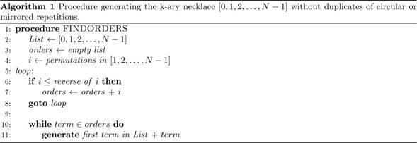
For instance, calling the above procedure with N = 5, FINDORDERS(5), would generate a list of permutations  with  length without  circular  or  mirrored  duplicates.   It should be realized that it is only a sufficient condition for routes being circular or mirrored duplicates to have same optimal E in Eq. 1; it is possible for routes not being repetitive on circular or mirrored orders to have same optimal value of E. It would be unrealistic to implement the above method for very large value N. If N = 25, there could be   ≈ 3.102 × 10²³ such different values of E to calculate, demanding unbearable computation time and memory. Because of this, a way of conquering this issue, Simulated Annealing and Metropolis Algorithm, comes into play.

 

2.2. Simulated Annealing and Metropolis Algorithm(SAMA)

The first idea of is Simulated Annealing Kirkpatrick  et al. (1983) could be based on the fact that minimizing a mathematical formula, such as Equation 1 is comparable to looking for a minimum energy state of a system in nature. There is a caution, however, in the nature of work with hot materials, known for a long time. In order to get a good crystallization, we need to cool down the material slowly, finding out its energy configuration of global minimum. On the other hand, if we cooled down the material too quickly, we might get glassy solids because we only reached the energy configuration of the “local” minimum for the material. Second, the nature of simulated annealing has the stochastic components, making it possible to assist in the asymptotic convergence analysis Emile et al. (1997).

First, we randomly generate an initial configuration of our system, then calculate the initial value of the quantity Ei. Then, because the system is ergodic, we randomly modify a little bit the configuration, calculating again the quantity after the change, say Ej. If the new quantity is smaller than the old one, we know that we find out a new configuration with smaller value of the quantity for which we would like to minimize. However, if the new quantity is larger than the old one, we may not be able to carelessly reject the new configuration. Because in this way we may “cool down” our system too quickly, possibly falling into the local minimum. The idea of Metropolis Algorithm is that when the new quantity in the new configuration is larger than the old one, instead of absolutely rejecting the new configuration, we make it possible to accept the new configuration by the following Metropolis probability:Newman (2013)

 

Equation 3

 

In practice, while randomly generating a number z between 0 and 1, we decide to accept the new configuration, with aid of Equation 3, if the random number z satisfies

 

z ≤ e^{−β(Ej−Ei)}; Equation 4

 

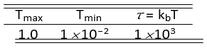
otherwise we reject the swap and return to the last tour order. To be more specific, throughout our study we have chosen the maximum temperature Tmax, minimum temperature Tmin, and τ = kbT as in Table 1

 

Table 1 Parameters used in SAMA.

 

Theoretically we may demonstrate that it is possible to find out the global minimum under infinite number of iterations. Emile et al. (1997) But it is not realistic to iterate infinitely number of times. Therefore, we need to compensate between the optimized value and time we need to consume. It is worth mentioning that in the optimization problem it is quite impossible to assure that we already reached the global minimum. All we can do is to find out another new solution to see if the new one out-reaches a smaller value compared with the old one.

 

2.3. Locations of Macao world heritage sites

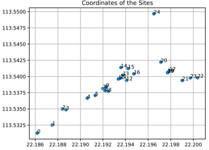
We collected our data about coordinates on latitudes and longitudes of the Macao World Heritage Sites from GOOGLE MAP, tabulated in Table A.1, with indications of names Emile et al. (1997). Figure 1 depicts the plot of site locations. Haversine formula Wikipedia of Haversine Formula, (2021) was used to convert from latitudes and longitudes to kilometers for a pair of sites.

 

Figure 1 Coordinates of sites with the Site ID number used throughout the paper, indicating name of every site in Table A.1. Site 17, 18, and 19 are too close to distinguish from one another.

 

3.    RESULTS AND DISCUSSIONS

We first compared the computation time between the brute-force method and SAMA. Later, for the first trial of SAMA, we introduced the latitudes and longitudes of the Macao World Heritage sites and calculated the optimal route with the minimum total distance by assuming that any pair of sites could be reached by a straight line. But this assumption is not realistic because in practice the real roads, streets or avenues in Macao are mostly not straight lines. Therefore, taking into consideration of real situations, for every pair of sites, we searched on GOOGLE MAP for the genuine time or distance required by either driving a car (Table A.2 or Table A.3), taking a bus (Table A.4), or  walking  across  the  streets  by  pedestrians(Table A.5 or Table A.6). Notice that GOOGLE MAP does not provide with data of distance for bus between pairs of sites. Data were tabulated in Appendix B to Appendix F. Through Table A.2 to Table A.6, number of Site ID at the left-hand column refers to the departure site, whereas number of Site ID on the top row refers to the destination site.

 

3.1. Comparison of computation time between the brute-force enumeration and SAMA on Fictitious Site Coordinates

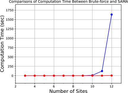
In order to compare time required by brute-force method and SAMA, we first randomly generate fictitious 12 sites, whose coordinates are lists in Table 2. Table 3 showed results of required computation time, after taking the average value on five times for each number of sites, under the condition of same shortest distance. It was evident that computation time for SAMA remained roughly less than 1 seconds for number of sites N less than 11, while for N = 12, 4.28 seconds. On the other hand, however, for the brute-force method, for fewer number of sites, the required time was less than that of SAMA, referring to the fact that for fewer number of sites, the brute-force method prevails SAMA. But the advantage of SAMA gradually appeared for larger N at least for two aspects. First, for N = 12, the brute-force method required roughly 1600 seconds to compute, while SAMA only required 4.28 seconds. The other advantage was that for larger number of N, brute-force method demands a lot of computer memory, causing it impractical to implement. Meanwhile, it is not a problem for SAMA because of the characteristic nature in randomly selecting the state of the system to compute. Figure 2 shows plots of required time vs. number of sites. It is obvious that demanding time for brute-force method increased dramatically for larger number of sites. Codes may be obtained via Ref. Brute Force vs. SAMA, Wei Shan Lee Github, (2021).

 

Table 2 Fictitious			coordinates of sites.
Sites ID	X	Y
0	0.428919706	0.361347607
1	0.530081873	0.698859005
2	0.635617396	0.45383111
3	0.164133133	0.584142242
4	0.255455144	0.797792439
5	0.700364502	0.329273766
6	0.38266615	0.280563838
7	0.524974098	0.349548083
8	0.24761384	0.628859237
9	0.30558778	0.083368041
10	0.816248668	0.079397349
11	0.413529397	0.340468561

 

Table 3 Comparisons of computation time, average on five times for each number of sites, between brute-force enumeration and SAMA. ⋆ shortest distance by either brute-force enumeration, or SAMA (a.u.). ⊛ computation time by SAMA (sec). Computer Specs were given in Figure 2 .
Number of Sites	⋆	⊚	⊛
3	0.84557967	∼ 0	∼ 0
4	1.22278990	0	0.25484419
5	1.36353451	0	0.25962210
6	1.55080373	0.00199866	0.23278880
7	1.67189785	0.01299381	0.76898718
8	1.67189945	0.11329699	0.61911297
9	1.70336830	1.37156701	0.81496930
10	2.06140792	9.85908175	0.64583468
11	2.55755845	122.93096805	0.93948197
12	2.55779639	1632.98429966	4.27968502

 

3.2. SAMA for two sites connected by a straight line

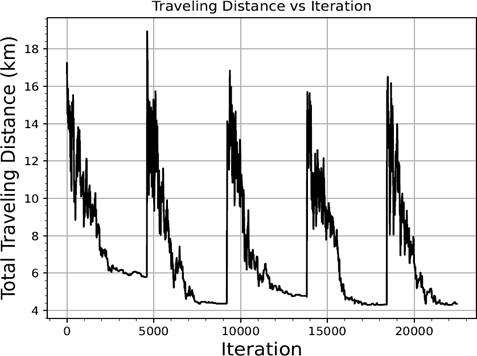
First, we randomly chose a site to be the origin and the end, initiating a tour path with a (perhaps high) value of total traveling distance. Afterward, SAMA cooled down the system, trying to find out a route with shorter total distance. Figure 3 showed the curve of total traveling distance vs. iteration.

Keeping in mind  that  instead  of  absolutely  rejecting  all  states with higher energy,  SAMA also allows a state with higher energy described by the rule in Equation 3, which is the reason for SAMA to put out the noisy curve within the iteration range 0 to 3000. Within Iteration 3000 to 5000, the curve remained relatively flat with the total distance roughly 6 km. Nevertheless, this could only be a local minimum for the particular initial condition.

To search for the global optimization, we started all over again by randomly initializing another starting point. This was shown at Iteration 4750 with a dramatically increase of the total traveling distance. SAMA would cool down the system again to reach another (probably) local minimum. We repeated the process until a targeted value of total distance was achieved. Codes may be obtained via Ref. SAMAV2, Wei Shan Lee Github, (2021).

 

Figure 2 Comparison of Computation Time between Brute-force enumeration(blue curve) and SAMA(red curve). Computer specs: Intel Core i7-4500U CPU @ 1.80 GHz 2.39 GHz. RAM 8GB. 64-bit operating system and x64-based processor.

Figure 3 Total traveling distance (km) vs. Iteration. For each loop of SAMA, the system was cooled down to the relatively flat curve, and then we initiated another state of system to repeat SAMA.

 

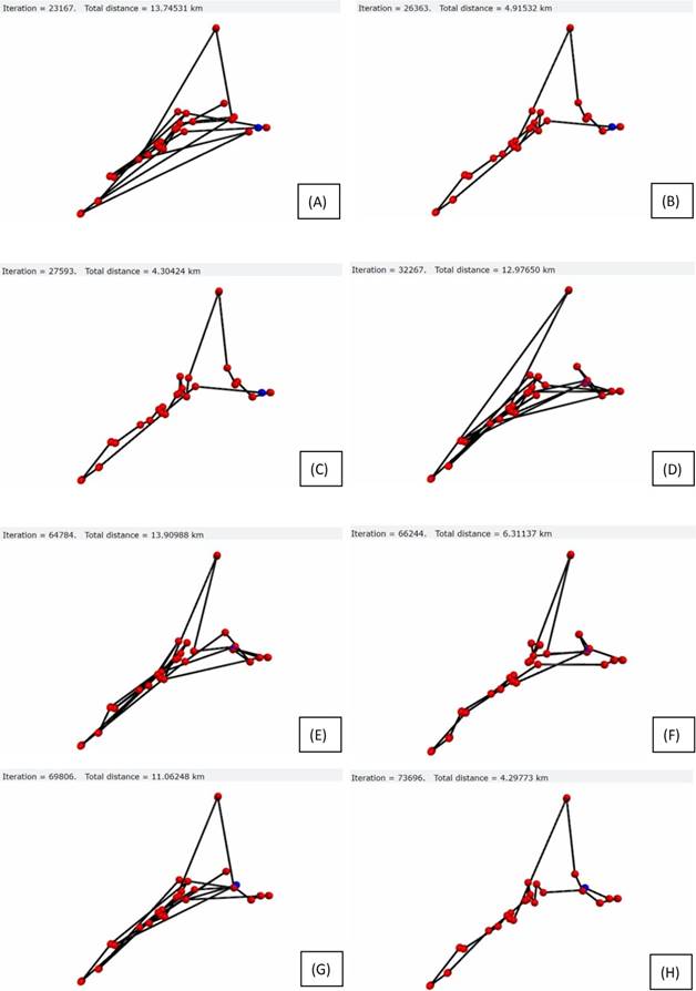
Figure 4 showed the snapshots of animation for some specific Iterations. The blue circle referred to the origin and the end for the specific route.  In Figure 4(A), for Iteration equal to 23167 with total distance 13.74 km, the snapshot showed messy connections among pairs of sites, meaning that the tour order has not yet been optimized. Immediately after this, at Iteration equal to 26363 with total distance 4.915 km, Figure 4(B) showed a much more organized route, which would later get improved in Figure 4(C) with a smaller value of total distance 4.3 km. Later, as shown in Figure 4(D) to Figure 4(F), we chose another site as the starting point and the end point. From Iteration 32267 to Iteration 66244, the total distances were reduced from 12.977 km to 6.311 km. Furthermore, we chose another site as the blue circle, as in Figure Figure 4(G). Finally, we reached to the targeted total distance 4.29773 km, acquiring the optimal route in Figure 4 (H) at Iteration 73696. Then the algorithm stopped. The whole animation video may be obtained in Ref Path Animation, Wei Shan Lee Github, (2021).

 

 

 

 

 

 

 

 

 

Figure 4 Snapshots of sightseeing order in the animations with various iterations, showing the total traveling distance at the specific iteration. The blue circle indicated the site of origin and the end for the particular route.

 

3.3. Optimal time or distance for all possible types of transportation

In order to calculate the optimal route with genuine least time or shortest distance, we collected, for each transportation method, the true value  of distance or time between a pair of sites with the form of matrices presented from Table A.2 to Table A.6 in Appendix B to Appendix F. It is worth nothing that the matrices in above Tables may not be symmetric, demonstrating the fact that some types of transportation have different routes between the same pair of sites. Afterward, we tabulated, in Table A.7, Table A.8, and Table A.9 in Appendix G, several routes that achieved optimal time or distance for every type of transportation. It should be understood without further notification that for each route, the circular or mirrored repetitions were also the optimal ones. In addition, in each type of transportation, the orders of optimal routes are either very similar or being circular or mirrored duplicates. For example, Table A.9a, Table A.9b, and Table A.9c show that in every of these three kinds of transportation, there is only one order of route that is not circular or mirrored duplicates. On the contrary, in Table A.7 and Table A.8, even if there are various optimal routes in these two types of transportation, the routes are quite similar in each kind of transportation.

At last, in Table 4 we may observe that it takes almost the same time for taking a bus (117 min), referring to Table A.9a, and on foot (115 min), referring to Table A.8. In spite of this, it takes shorter distance on foot (7.844 km), referring to Table A.9b, than by driving a car (13.916 km), referring to Table A.9c. Codes may be retrieved via Ref SAMAV3, Wei Shan Lee Github, (2021). These results suggest that the traffic condition in Macao imminently acquires improvement. The average computation time was taken by calculating the mean computation time of five routes in each transportation. Time demanded for computation ranged from 5 minutes (for least time on foot) to 74 minutes (for shortest distance by car). There seemed no clear pattern or tendency in types of transportation for the reason why required time for computing the optimal routes were different.

Table 4 Comparison of all types of transportation, including driving a car, taking a bus, or on foot. Computer Spec is given in the caption of Figure 2
Types of transportation		Least time (min)		Shortest distance (km)		Average computation time for the optimal value (min : sec)
					Least time		Shortest Distance
Car	78		13.916		10:34		74:25:00
Bus	117		Not Available		44:39:00		Not Available
Pedestrian	115		7.844		05:19		33:25:00

 

4.    CONCLUSIONS AND RECOMMENDATIONS

We made use of Simulated Annealing and Metropolis Algorithm (SAMA) to obtain optimal sightseeing orders for least time or shortest distance of Macao World Heritage Sites with actual time or distance values between a pair of sites. Without repeating any site while completing a loop of the historical remains in Macao, the optimal least time for driving a car could be 78 min, while taking a bus would be 117 min, and 115 min on foot. On the other hand, the optimal shortest distance by

car would be 13.916 km, while on foot, 7.844 km. This manifests the terrible traffic condition in the city of Macao, where improvement on public transportation is imperative.

Also, we provided a simple algorithm to generate the k-ary necklace. Based on this, we calculated computation time required in the brute-force method to obtain the optimal time or distance by enumerating all possible routes. Whereas for small number of sites, the brute- force enumeration performed much faster in calculating the optimal value, SAMA prevailed when number of sites increased. In our study, we demonstrated that when number of sites was 12, SAMA only required 3 orders of magnitude less in time than the brute-force method to obtain the optimal total distance.

At last, we provided several optimal routes in different kinds of transportation for tourists in Macao, from which choices may be made to manage their visiting plans more efficiently.

 

5.    ACKNOWLEDGEMENTS

We thank Pui Ching Middle School in Macao PRC for the kindness to support this research project.

 

6.    APPENDICES (if applicable)

 

Appendix A           Locations of Macao World Heritage Sites
Site ID	Latitude	Longitude	Name
0	22.18618015	113.5312755	Templo de A-Ma
1	22.18749972	113.5325193	Quartel dos Mouros
2	22.1884061	113.5349956	Largo do Lilau
3	22.1887227	113.5348891	Casa do Mandarim
4	22.19061015	113.5366617	Igreja de S˜tildea o Louren¸co
5	22.19131257	113.537089	Igreja do Semin´ario de S˜ao Jos´e
6	22.19218864	113.5378323	Largo de Santo Agostinho
7	22.19199551	113.5381535	Teatro Dom Pedro V
8	22.19247942	113.5376891	Biblioteca Sir Robert Ho Tung
9	22.19228218	113.5383978	Igreja de Santo Agostinho
10	22.19336355	113.5396164	Instituto para os Assuntos Municipais
11	22.19354689	113.5397601	Largo do Senado
12	22.19407548	113.5394111	Templo de Sam Kai Vui Kun
13	22.19374817	113.5402032	Santa Casa da Miserico´rdia de Macau
14	22.19358846	113.5413864	Igreja da S´e Catedral
15	22.19422634	113.5412314	Casa de Lou Kau
16	22.19473103	113.540409	Igreja de S˜ao Domingos
17	22.19788781	113.5408688	Ru´ınas de S˜ao Paulo
18	22.19774218	113.540654	Templo de Na Tcha
19	22.19772073	113.5405832	Old Macau City Walls Sections
20	22.19712896	113.5422227	Monte do Forte
21	22.19901644	113.5393853	Igreja de Santo Antˆonio  de Lisboa
22	22.20036032	113.5398153	Funda¸c˜ao Oriente
23	22.1997325	113.5397974	Cemit´erio Protestante
24	22.19650437	113.5496706	Farol e Fortaleza da Guia
A.1: Site ID, latitude, longitude, and names of the Macao World Heritage Sites. Data retrieved from GOOGLE MAP.

 

Appendix B             Car Driving time for Pairs of Sites
	0	1	2	3	4	5	6	7	8	9	10	11	12	13	14	15	16	17	18	19	20	21	22	23	24
0	0	7	6	6	7	6	8	9	8	9	8	8	8	8	8	10	10	13	13	13	14	11	15	12	11
1	4	0	7	7	6	7	9	9	8	9	9	9	10	10	9	11	12	14	14	14	14	11	15	12	11
2	4	2	0	1	4	4	6	6	6	5	5	5	6	6	5	6	6	9	9	9	10	8	11	8	9
3	5	1	1	0	9	9	10	11	10	10	9	9	10	9	9	11	11	14	14	14	14	12	17	13	11
4	5	3	2	1	0	1	3	4	3	4	4	4	5	5	4	6	6	9	9	9	9	6	9	7	7
5	9	6	5	5	4	0	2	2	2	2	5	5	5	5	5	7	7	9	9	9	10	6	9	6	8
6	7	4	3	3	2	1	0	1	3	1	3	3	5	4	3	5	5	8	8	8	8	6	9	7	7
7	6	4	3	3	2	1	3	0	3	1	3	3	5	4	4	5	5	8	8	8	9	6	9	7	7
8	7	5	4	4	2	2	1	1	0	1	4	4	5	4	4	6	6	10	11	11	12	6	8	7	8
9	6	4	3	3	2	1	3	4	3	0	3	3	5	4	3	5	5	8	8	8	8	6	9	7	6
0	9	8	7	8	7	7	5	5	5	5	0	1	1	3	2	5	5	9	9	9	9	4	8	4	5
11	9	8	7	7	7	7	6	6	6	6	1	0	2	3	2	5	5	7	7	7	7	4	7	5	6
12	11	10	9	9	7	8	6	7	6	6	4	4	0	8	7	10	10	9	9	9	10	3	7	4	11
13	16	15	14	14	13	13	14	14	14	14	12	12	14	0	1	4	4	9	9	9	9	12	13	12	7
14	16	15	13	13	13	12	14	14	14	14	11	11	12	1	0	3	3	8	7	7	8	11	11	11	6
15	16	14	13	13	12	12	13	13	13	13	11	11	12	11	10	0	1	8	8	8	8	11	12	11	7
16	16	14	13	13	12	12	13	14	13	13	10	10	12	11	11	1	0	8	8	8	9	11	13	12	7
17	20	19	18	18	16	16	15	15	15	15	15	15	15	16	15	11	11	0	1	1	10	4	11	4	12
18	19	18	18	17	16	16	15	15	15	15	15	15	15	15	15	11	11	1	0	1	9	4	10	4	12
19	23	21	20	20	18	16	16	17	16	16	15	15	16	15	15	11	11	1	1	0	9	4	10	5	12
20	14	12	12	11	10	10	11	12	11	12	9	9	10	9	9	2	2	7	7	7	0	10	11	10	5
21	18	16	16	15	14	14	13	13	13	13	13	13	13	12	11	8	8	6	6	6	6	0	7	1	8
22	18	16	15	15	13	13	11	12	11	11	11	11	11	13	13	8	8	6	6	6	6	9	0	10	9
23	19	18	17	17	15	15	17	17	16	15	13	13	15	13	13	9	9	6	6	6	6	9	8	0	9
24	12	11	10	9	9	9	11	11	10	11	8	8	9	8	7	9	9	7	7	7	7	10	12	11	0
A.2: Car driving time (in units of minutes) for pairs of sites. The Site ID number is given in Table A.1. Site ID numbers at the left-hand side column mean the departure site, while Site ID numbers at the top row refer to the destination site.

 

Appendix C                    Car Driving distance for Pairs of Sites
	0	1	2	3	4	5	6	7	8	9	10	11	12	13	14	15	16	17	18	19	20	21	22	23	24
0	0	1.9	1.6	1.6	1.8	1.8	2.2	2.2	2.1	2.2	2.1	2.1	2.3	2.3	2.1	2.6	2.6	3.4	3.4	3.5	3.5	3.5	3.7	3.6	4.7
1	1.3	0	2.5	2.2	2.8	2.7	3.5	3.5	3.1	3	3.3	3.3	3.5	3.5	3.3	3.8	3.8	4.7	4.7	4.8	4.7	4.7	4.5	4.4	5.1
2	1.2	0.3	0	0.65	0.9	0.9	1.3	1.3	1.2	1.2	1.2	1.2	1.4	1.4	3.1	3.6	3.6	4.9	4.9	4.9	4.8	4.8	2.8	2.2	2.4
3	1.6	0.3	0.065	0	3.1	3	3.4	3.4	3.4	3.3	3.3	3.6	3.8	3.8	3.8	4.1	4.1	5	5	5.1	5	5	4.8	2.2	4.8
4	1.5	0.6	0.35	0.065	0	0.3	0.7	0.7	0.6	0.7	0.85	0.85	1.05	1.05	0.85	1.4	1.4	2.2	2.2	2.3	2.3	2.3	2.2	1.6	2.1
5	2.2	1.4	1.1	1.1	0.8	0	0.4	0.4	0.3	0.4	0.55	0.55	1.2	1.2	1.1	1.6	1.6	2.3	2.3	2.4	2.4	2.4	1.9	1.3	2.3
6	1.9	1	0.75	0.75	0.4	0.4	0	0.026	0.7	0.32	0.65	0.65	0.85	0.85	0.7	1.2	1.2	2	2	2.1	2.1	1.6	2.3	1.7	1.9
7	1.8	1	0.75	0.75	0.4	0.4	0.75	0	0.7	0.32	0.65	0.65	0.85	0.85	0.7	1.2	1.2	2	2	2.1	2.1	1.6	2.3	1.7	1.9
8	2	1.1	0.85	0.7	0.5	0.5	0.11	0.14	0	0.14	0.5	0.75	1	1	0.8	1.3	1.3	2.1	2.1	2.2	2.2	1.1	1.7	1.2	2
9	1.8	1	0.7	0.55	0.35	0.35	0.7	0.75	0.65	0	0.75	1	1.25	1.25	1.05	1.2	1.2	2	2	2.1	2.1	1.5	2.2	1.6	1.8
0	2.4	1.6	1.4	1.4	1.3	1.3	1.1	1.2	1.1	1.2	0	0.005	0.21	0.21	0.4	0.85	0.85	1.8	1.8	1.9	1.9	0.9	1.7	1	1.6
11	2.4	1.6	1.4	1.4	1.3	1.3	1.1	1.2	1.1	1.2	1.2	0	0.21	0.21	0.4	0.9	0.9	1.8	1.8	1.9	1.9	0.9	1.7	1	1.6
12	3	2.3	2	2	1.7	1.7	1.5	1.5	1.4	1.5	1.5	0.8	0	1.3	0.4	1.7	1.7	1.9	1.9	2	2	1	1.4	0.9	2.4
13	3.7	3	2.8	2.8	2.4	2.4	2.8	2.8	2.7	2.8	2.8	2	2.2	0	0.16	0.65	0.65	1.5	1.5	1.6	1.6	2.1	2.5	2.2	1.4
14	3.6	2.9	2.6	2.6	2.3	2.3	2.6	2.6	2.5	2.6	2.6	1.8	2	0.16	0	0.5	0.5	1.4	1.4	1.4	1.4	1.9	2.4	2	1.2
15	3.9	3.2	2.9	2.9	2.6	2.6	2.9	2.9	2.8	2.9	2.9	2.1	2.3	0.36	2.2	0	0.68	1.7	1.7	1.8	1.8	2.3	2.7	2.3	1.5
16	3.9	3.2	2.9	2.9	2.6	2.6	2.9	2.9	2.8	2.9	2.9	2.1	2.3	0.36	2.2	0.068	0	1.7	1.7	1.8	1.8	2.3	2.7	2.3	1.5
17	4.8	4.1	3.8	3.8	3.6	3.6	3.4	3.4	3.3	3.4	3.4	3.6	3.1	3.3	3.1	2.2	2.2	0	0	0.007	1.8	0.55	2.1	0.7	2.4
18	4.7	4	3.7	3.7	3.4	3.4	3.3	3.3	3.2	3.3	3.3	3.5	3	3.2	3	2.1	2.1	0	0	0.007	1.8	0.55	2.1	0.7	2.4
19	4.8	4.1	4	4	3.5	3.5	3.4	3.4	3.3	3.4	3.4	2.6	3.1	3.3	3.1	2.2	2.2	0.1	0.1	0	1.8	0.6	2.1	0.7	2.4
20	3.5	2.8	2.6	2.6	2.3	2.3	2.2	2.2	2.5	2.2	2.2	1.4	2	2.1	1.9	0.45	0.45	1.3	1.3	1.4	0	1.9	2.4	2	1.2
21	4.2	3.5	3.4	3.4	2.9	2.9	2.8	2.8	2.7	2.8	2.8	2	2.6	2.7	2.6	1.7	1.7	1.1	1.1	1.2	1.2	0	1.5	0.12	1.8
22	4.2	3.4	3.1	3.1	2.8	2.8	2.6	2.6	2.5	2.6	2.6	1.8	2.4	2.5	2.5	1.7	1.7	1.1	1.1	1.2	1.2	1.7	0	1.8	1.8
23	4.3	3	3.4	3.4	3	3	2.9	2.9	2.8	2.9	2.9	2.1	2.7	2.8	2.6	1.7	1.7	1.2	1.2	1.2	1.2	1.7	1.6	0	1.9
24	4.3	3.1	3.5	3.5	2.1	2.1	2.4	2.4	2.3	2.4	2.4	1.6	2.2	2.3	1.7	1.8	1.8	1.5	1.5	1.6	1.6	2	2.5	2.1	0

A.3:  Car driving distance (in units of km) for pairs of sites.  The Site ID number is given in Table  A.1.  Site ID numbers at the left-hand side column mean the departure site, while Site ID numbers at the top row refer to the destination site.

 

 

Appendix D                   Bus Driving time for Pairs of Sites
	0	1	2	3	4	5	6	7	8	9	10	11	12	13	14	15	16	17	18	19	20	21	22	23	24
0	0	4*	34	8*	23	25	25	24	27	24	25	26	26	26	27	28	30	31	31	35	35	30	34	32	39
1	4*	0	4*	4*	31	30	27	26	28	26	26	26	26	27	21	22	23	28	28	30	27	31	32	31	36
2	12	4*	0	1*	4*	7*	28	27	30	27	23	23	24	24	17	23	24	28	28	37	28	34	36	35	32
3	12	4*	1*	0	4*	6*	28	27	29	27	22	22	24	24	22	23	24	28	28	36	27	34	36	35	31
4	14	13	10	10	0	2*	4*	5*	6*	5*	22	23	24	23	21	23	24	28	28	31	27	22	25	23	30
5	16	15	13	12	2*	0	5*	4*	4*	4*	6*	6*	6*	7*	23	25	9*	11*	11*	35	27	20	22	20	32
6	19	18	18	18	4*	5*	0	1*	1*	1*	4*	4*	4*	4*	6*	6*	6*	10*	10*	25	21	17	19	17	28
7	18	16	17	17	5*	4*	1*	0	2*	1*	4*	4*	5*	5*	6*	7*	7*	11*	11*	26	20	18	20	19	28
8	18	19	20	19	6*	4*	1*	2*	0	2*	3*	4*	4*	5*	6*	6*	6*	10*	10*	13*	23	18	19	18	31
9	18	16	17	17	5*	4*	1*	1*	2*	0	4*	4*	5*	5*	6*	7*	7*	11*	11*	26	21	18	20	19	29
0	19	21	21	20	25	6*	4*	4*	3*	4*	0	1*	1*	1*	3*	3*	3*	7*	7*	10*	11*	15	17	16	28
11	19	21	20	20	24	6*	4*	4*	4*	4*	1*	0	1*	1*	3*	3*	3*	7*	7*	10*	11*	16	16	18	27
12	19	20	19	19	18	6*	5*	5*	5*	5*	1*	1*	0	2*	3*	3*	3*	6*	6*	9*	10*	14	17	15	27
13	21	22	22	21	21	8*	6*	6*	6*	6*	2*	2*	2*	0	2*	2*	2*	6*	6*	9*	10*	15	18	16	27
14	21	20	18	18	18	21	7*	7*	7*	7*	3*	3*	3*	2*	0	1*	2*	6*	6*	9*	8*	16	18	17	25
15	22	22	21	21	20	10*	7*	7*	7*	8*	3*	3*	3*	2*	1*	0	1*	5*	5*	8*	8*	15	17	16	27
16	23	23	23	21	21	10*	7*	8*	7*	8*	4*	4*	3*	2*	3*	1*	0	5*	5*	7*	7*	15	18	16	28
17	22	23	23	24	20	12*	11*	11*	11*	11*	7*	7*	6*	6*	6*	5*	4*	0	1*	2*	10*	3*	6*	5*	32
18	22	23	23	23	20	11*	11*	11*	10*	11*	7*	7*	6*	5*	6*	4*	4*	1*	0	1*	10*	3*	6*	5*	32
19	25	26	26	26	23	14*	14*	14*	13*	14*	10*	10*	9*	8*	9*	7*	7*	2*	1*	0	10*	6*	9*	8*	38
20	26	25	23	23	23	26	13*	13*	13*	23	9*	9*	8*	8*	6*	6*	5*	9*	9*	9*	0	20	22	20	29
21	21	22	22	21	18	17	16	16	16	17	12	12	8*	9*	9*	8*	7*	4*	4*	7*	13*	0	2*	1*	31
22	25	24	24	23	21	21	20	20	19	21	18	17	16	19	22	10*	9*	6*	6*	9*	14*	2*	0	1*	32
23	24	23	23	22	19	19	19	18	18	19	15	15	9*	10*	11*	9*	8*	5*	5*	8*	13*	1*	1*	0	30
24	32	31	31	31	29	30	29	29	29	30	26	25	25	26	25	25	25	29	29	18*	26	26	27	26	0
A.4: Bus driving time (in units of minutes) for pairs of sites. If, for a pair of sites, there is no suggested route for bus that may be found from the google map, then the value is replaced with the least time for the pedestrians to walk across the two sites,  indicated with ⋆.  The Site ID number is given in Table A.1. Site ID numbers at the left-hand side column mean the departure site, while Site ID numbers at the top row refer to the destination site.

 

Appendix E         Pedestrian walking time for Pairs of Sites
	0	1	2	3	4	5	6	7	8	9	10	11	12	13	14	15	16	17	18	19	20	21	22	23	24
0	0	4	8	8	12	13	16	16	16	14	18	18	19	19	18	20	21	24	24	27	25	23	26	24	35
1	4	0	4	4	8	10	12	12	13	11	15	15	16	16	15	17	18	22	22	25	22	24	26	25	32
2	8	4	0	1	4	7	9	9	10	8	12	12	13	13	13	14	16	19	19	22	19	21	23	22	30
3	8	4	1	0	4	6	9	8	10	8	12	12	13	13	12	13	15	19	19	22	19	20	22	21	29
4	12	8	4	4	0	3	6	5	7	4	8	9	9	10	9	10	12	15	14	17	16	17	19	18	26
5	13	10	7	6	3	0	5	5	4	4	7	7	7	9	9	10	10	12	12	15	14	14	17	16	25
6	16	12	9	9	6	5	0	1	2	4	4	4	5	6	7	8	8	11	11	14	13	14	16	15	23
7	16	12	9	8	5	5	1	0	2	1	5	4	6	7	7	8	8	12	11	14	14	14	17	16	24
8	16	13	10	10	7	4	2	2	0	2	4	4	5	6	7	8	8	11	11	14	13	13	16	15	24
9	14	11	8	8	4	4	1	1	2	0	5	5	6	7	7	8	8	12	12	14	14	14	17	16	24
0	18	15	12	12	8	7	4	5	4	5	0	1	2	2	3	4	4	8	7	10	9	10	15	11	17
11	18	15	12	12	9	7	4	4	4	5	1	0	1	2	3	4	4	7	7	10	9	10	13	11	20
12	19	16	13	13	9	7	5	6	5	6	2	1	0	3	4	3	3	6	6	9	8	9	11	10	19
13	19	16	13	13	10	9	6	7	6	7	2	2	3	0	2	2	3	6	6	9	8	9	12	10	18
14	18	15	13	12	9	9	7	7	7	7	3	3	4	2	0	2	3	7	7	9	7	10	12	11	17
15	20	17	14	13	10	10	8	8	8	8	4	4	3	2	2	0	2	5	4	8	6	8	11	9	17
16	21	18	16	15	12	10	8	8	8	8	4	4	3	3	3	2	0	4	5	7	6	8	10	9	17
17	24	22	19	19	15	12	11	12	11	12	8	7	6	6	7	5	4	0	1	3	9	5	7	6	19
18	24	22	19	19	14	12	11	11	11	12	7	7	6	6	7	5	4	1	0	1	9	7	7	6	19
19	27	25	22	22	17	15	14	14	14	14	10	10	9	9	9	8	7	3	1	0	9	7	10	9	19
20	25	22	19	19	16	14	13	14	13	14	9	9	8	8	7	6	6	9	9	9	0	13	15	13	17
21	23	24	21	20	17	14	14	14	13	14	10	10	9	9	10	8	8	5	7	7	13	0	2	1	21
22	26	26	23	22	19	17	16	17	16	17	15	13	11	12	12	11	10	7	7	10	15	2	0	2	22
23	24	25	22	21	18	16	15	16	15	16	11	11	10	10	11	9	9	6	6	9	13	1	2	0	21
24	35	32	30	29	26	25	23	24	24	24	17	20	19	18	17	17	17	19	19	19	17	21	22	21	0
A.5: Pedestrian walking time (in units of minutes) for pairs of sites. The Site ID number is given in Table A.1. Site ID numbers at the left-hand side column mean the departure site, while Site ID numbers at the top row refer to the destination site.

 

Appendix F   Pedestrian walking distance for Pairs of Sites
	0	1	2	3	4	5	6	7	8	9	10	11	12	13	14	15	16	17	18	19	20	21	22	23	24
0	0	0.24	0.55	0.55	0.85	1	1.1	1.1	1.2	1.1	1.3	1.3	1.5	1.4	1.4	1.5	1.6	1.9	1.9	2.1	1.9	1.8	2	1.9	2.6
1	0.24	0	0.3	0.3	0.6	0.75	0.9	0.85	1	0.85	1.1	1.1	1.2	1.2	1.2	1.2	1.4	1.7	1.6	1.8	1.7	1.8	2	1.9	2.4
2	0.55	0.3	0	0.064	0.35	0.5	0.65	0.6	0.75	0.6	0.85	0.85	0.95	0.9	0.9	1	1.1	1.4	1.4	1.6	1.4	1.6	1.8	1.7	2.2
3	0.55	0.3	0.064	0	0.3	0.5	0.6	0.6	0.75	0.6	0.85	0.85	0.95	0.9	0.9	0.95	1.1	1.4	1.4	1.6	1.4	1.5	1.7	1.6	2.1
4	0.85	0.6	0.35	0.3	0	0.18	0.4	0.35	0.5	0.35	0.6	0.6	0.65	0.65	0.65	0.75	0.9	1.1	1.1	1.2	1.2	1.2	1.4	1.3	1.9
5	1	0.75	0.5	0.5	0.18	0	0.4	0.35	0.3	0.35	0.45	0.45	0.5	0.55	0.65	0.7	0.7	0.9	0.9	1.1	1	1.1	1.3	1.1	1.9
6	1.1	0.9	0.65	0.6	0.4	0.4	0	0.026	0.11	0.032	0.25	0.25	0.3	0.4	0.45	0.5	0.5	0.8	0.8	1	0.85	1	1	1.1	1.6
7	1.1	0.85	0.6	0.6	0.35	0.35	0.026	0	0.14	0.005	0.28	0.27	0.28	0.4	0.45	0.5	0.55	0.85	0.8	1	0.9	1	1.2	1.1	1.7
8	1.2	1	0.75	0.75	0.5	0.3	0.11	0.14	0	0.14	0.27	0.27	0.35	0.4	0.5	0.5	0.5	0.8	0.75	1	0.9	0.95	1.1	1	1.7
9	1.1	0.85	0.6	0.6	0.35	0.35	0.032	0.005	0.14	0	0.28	0.28	0.35	0.4	0.45	0.55	0.55	0.85	0.8	1	0.9	1	1.2	1.1	1.7
0	1.3	1.1	0.85	0.85	0.6	0.45	0.25	0.28	0.27	0.28	0	0.005	0.11	0.12	0.22	0.27	0.3	0.6	0.6	0.8	0.65	0.8	1	0.9	1.4
11	1.3	1.1	0.85	0.85	0.6	0.45	0.25	0.27	0.27	0.28	0.005	0	0.11	0.12	0.22	0.27	0.29	0.6	0.6	0.75	0.65	0.8	1	0.9	1.4
12	1.5	1.2	0.95	0.95	0.65	0.5	0.3	0.28	0.35	0.35	0.11	0.11	0	0.2	0.26	0.24	0.25	0.5	0.5	0.7	0.6	0.7	0.85	0.75	1.4
13	1.4	1.2	0.9	0.9	0.65	0.55	0.4	0.4	0.4	0.4	0.12	0.12	0.2	0	0.18	0.18	0.22	0.5	0.5	0.7	0.65	0.75	0.9	0.8	1.4
14	1.4	1.2	0.9	0.9	0.65	0.65	0.45	0.45	0.5	0.45	0.22	0.22	0.26	0.18	0	0.12	0.22	0.5	0.5	0.7	0.5	0.75	0.95	0.85	1.2
15	1.5	1.2	1	0.95	0.75	0.7	0.5	0.5	0.5	0.55	0.27	0.27	0.24	0.18	0.12	0	0.12	0.4	0.4	0.6	0.5	0.65	0.85	0.75	1.3
16	1.6	1.4	1.1	1.1	0.9	0.7	0.5	0.55	0.5	0.55	0.3	0.29	0.25	0.22	0.22	0.12	0	0.4	0.35	0.55	0.45	0.65	0.85	0.7	1.3
17	1.9	1.7	1.4	1.4	1.1	0.9	0.8	0.85	0.8	0.85	0.6	0.6	0.5	0.5	0.5	0.4	0.4	0	0.008	0.23	0.65	0.35	0.5	0.4	1.3
18	1.9	1.6	1.4	1.4	1.1	0.9	0.8	0.8	0.75	0.8	0.6	0.6	0.5	0.5	0.5	0.4	0.35	0.008	0	0	0.65	0.3	0.5	0.4	1.3
19	2.1	1.8	1.6	1.6	1.2	1.1	1	1	1	1	0.8	0.75	0.7	0.7	0.7	0.6	0.55	0.23	0	0	0.7	0.55	0.7	0.6	1.3
20	1.9	1.7	1.4	1.4	1.2	1	0.85	0.9	0.9	0.9	0.65	0.65	0.6	0.65	0.5	0.5	0.45	0.65	0.65	0.7	0	0.85	0.95	0.85	1.1
21	1.8	1.8	1.6	1.5	1.2	1.1	1	1	0.95	1	0.8	0.8	0.7	0.75	0.75	0.65	0.65	0.35	0.3	0.55	0.85	0	0.19	0.094	1.5
22	2	2	1.8	1.7	1.4	1.3	1	1.2	1.1	1.2	1	1	0.85	0.9	0.95	0.85	0.85	0.5	0.5	0.7	0.95	0.19	0	0.13	1.6
23	1.9	1.9	1.7	1.6	1.3	1.1	1.1	1.1	1	1.1	0.9	0.9	0.75	0.8	0.85	0.75	0.7	0.4	0.4	0.6	0.85	0.094	0.13	0	1.5
24	2.6	2.4	2.2	2.1	1.9	1.9	1.6	1.7	1.7	1.7	1.4	1.4	1.4	1.4	1.2	1.3	1.3	1.3	1.3	1.3	1.1	1.5	1.6	1.5	0
A.6: Pedestrian walking distance (in units of km) for pairs of sites. The Site ID number is given in Table A.1. Site ID numbers at the left-hand side column mean the departure site, while Site ID numbers at the top row refer to the destination site.

 

Appendix G                 Several Optimal Routes for Each Possible Transportation
Route 1	Route 2	Route 3	Route 4	Route 5		Route 1	Route 2	Route 3	Route 4	Route 5
17	23	19	10	0		23	1	19	17	8
18	22	17	12	13		21	2	17	18	11
19	20	21	6	14		17	4	21	19	12
21	24	23	5	15		19	9	22	21	16
23	4	22	8	16		18	7	23	22	17
22	3	20	7	18		16	6	24	23	18
20	2	15	9	17		12	10	20	24	19
24	1	16	4	19		11	13	16	20	21
11	0	24	2	21		6	14	12	15	22
10	5	11	3	23		7	15	11	14	23
12	8	10	1	22		9	20	6	13	24
9	6	12	0	20		4	24	7	10	20
5	7	9	13	24		3	22	9	8	15
8	9	5	14	11		2	23	4	5	14
6	10	8	15	10		1	21	2	4	13
7	12	6	16	12		0	19	1	2	10
4	11	7	19	8		5	18	0	3	6
3	13	4	18	6		8	17	3	1	7
2	14	2	17	5		10	16	5	0	9
1	15	3	21	7		13	12	8	9	4
0	16	1	23	9		14	11	10	6	2
13	17	0	22	4		15	8	13	7	1
14	19	13	20	3		20	5	14	11	0
15	18	14	24	2		24	3	15	12	3
16	21	18	11	1		22	0	18	16	5
17	23	19	10	0		23	1	19	17	8
A.7:  Optimal time (78 min) by car.               A.8: Optimal time (115 min) on foot.

 

 

 

 

Route			Route			Route
19			20			17
18			16			18
17			15			19
23			14			21
22			13			23
21			11			20
0			10			16
1			12			15
2			7			13
3			9			14
4			6			24
5			8			5
7			5			8
9			4			6
6			3			7
8			2			9
10			1			4
12			0			3
11			21			2
13			22			1
14			23			0
15			17			10
16			18			11
20			19			12
24			24			22
19			20			17
(a)			(b)			(c)
A.9: Optimal routes for: A.9a shortest time by bus (117 min), A.9b on foot (7.844 km), and A.9c shortest distance by car (13.916 km).

 

REFERENCES

B. Guenin, J. KoneMann, and L. Tuncel (2014), A gentle Introduction to Optimization, Cam- bridge University Press.  Retrived from https://doi.org/10.1017/CBO9781107282094

C. Rossant (2018), IPython Interactive Computing and Visualization Cookbook, 2nd Ed., Packt Publishing, pp 481-486.

E. L. Lawler (1985), The Travelling Salesman Problem: A Guided Tour of Combinatorial Opti- mization (Repr. with corrections. ed.). John Wiley & sons. ISBN 978-0471904137.

Emile H.L. Aarts, Jan H.M. Korst, Peter J.M. van Laarhoven (1997), "Simulated Annealing", Local Search in Combinatorial Optimization. Edited by E. Aarts and J.K. Lenstra, John Wiley & Sons Ltd, pp 91-120. Retrieved from https://doi.org/10.2307/j.ctv346t9c.9

Fei Liu and GuangZhou Zeng (2009), "Study of genetic algorithm with reinforcement learning to solve the TSP ", Expert Systems with Applications, Volume 36, Issue 3, Part 2, April, pp 6995-7001.  Retrieved from https://doi.org/10.1016/j.eswa.2008.08.026

G. Dantzig, R. Fulkerson, and S. Johnson (1954), "Solution of a Large Scale Traveling Salesman Problem", Rand Paper, P-510. Retrieved from https://www.rand.org/pubs/papers/P510.html

J. Sawada (2003), "A fast algorithm to generate necklaces with fixed content", Theoretical Computer Science, 301, 477-489. Retrieved from https://doi.org/10.1016/S0304-3975(03)00049-5

Jon Jouis Bentley (1992), "Fast Algorithms for Geometric Traveling Salesman Problems", In- forms Journal on Computing, Vol. 4, pp. 357-452. Retrieved from https://doi.org/10.1287/ijoc.4.4.387

M.S. Tarkov (2015), "Solving the traveling salesman problem using a recurrent neural network", Numerical Analysis and Applications volume 8, pp. 275-283. Retrieved from https://doi.org/10.1134/S1995423915030088

Mark Newman (2013), Computational Physics, Revised and Expanded 2013. ISBN 978- 148014551-1. pp. 490-492.

Merrill M. Flood (1956), "The Traveling-Salesman Problem", Operations Research, Vol. 4, pp. 1- 137,. Retrieved from https://doi.org/10.1287/opre.4.1.61

N Mazyavkina, S. Sviridov, S. Ivanov, and E. Burnaev (2020), "Reinforcement Learning for Combinatorial Optimization: A Survey", arXiv:2003.03600v3. Retrieved from https://arxiv.org/pd f/2003.03600

Ottoni, A.L.C., Nepomuceno, E.G., Oliveira, M.S.d. et al (2021). Reinforcement learning for the traveling salesman problem with refueling. Complex Intell. Syst.. Retrieved from https://doi.org/10.1007/s40747-021-00444-4

S. Kirkpatrick, C. D. Gelatt Jr., and M. P. Vecchi (1983), "Optimization by Simulated Anneal- ing", Science, Vol. 220, pp. 671-680. Retrieved from https://doi.org/10.1126/science.220.4598.671

Stephen. P. Bradley (1977), Arnoldo C. Hax, and Thomas, L. Magnanti, Applied Mathematical Programming, Addison-Wesley Publishing Company Inc.

Wikipedia of Global Optimization 2021, https://en.wikipedia.org/wiki/Global_optimization

Wikipedia of Haversine Formula, (2021). Retrieved from https://en.wikipedia.org/wiki/Haversine_formula

Wikipedia of Historical Centre of Macau (2021) Retrieved from https://en.wikipedia.org/wiki/Historic_Centre_of_Macau

Wikipedia of Macau Wiki, (2021) Retrieved from https://en.wikipedia.org/wiki/Macau

SAMAV2, Wei Shan Lee Github, (2021) Retrieved from https://github.com/weishanlee/SAMAV2_2

Path Animation, Wei Shan Lee Github, (2021) Retrieved from https://github.com/weishanlee/SAMAV2_2/tree/main/4.29773

SAMAV3, Wei Shan Lee Github, (2021) Retrieved from https://github.com/weishanlee/SAMAV3_1

Brute Force vs. SAMA, Wei Shan Lee Github, 2021 Retrieved from https://github.com/weishanlee/brute-force-vs-simulated-annealing-metropolisalgorithm

Stackoverflow, 51531766 , 2018. Retrieved  from https://stackoverflow.com/questions/51531766/python-algorithms-necklace-generation- circular-permutations

Stackoverflow, 960557, 2009. Retrieved from https://stackoverflow.com/questions/960557/how-to-generate-permutations-of-a-list- without-reverse-duplicates-in-python-us

Macao Gov. Tourism Office, 2021. Retrieved from https://www.macaotourism.gov.mo/zh-hant/sightseeing/macao-world-heritage

Statista, 319153, (2020) https://www.statista.com/statistics/319153/macau-visitor-arrivals/ Note that in 2020 the number of visitors dropped significantly to 5.9 millions because of the COVID-19 outbreak.

Cultural Affairs Bureau (2021), Retrieved from https://www.wh.mo/en/site/