Integrating Carrying Capacity and War Dynamics into Richardson’s Arms Race Model: An Analytic Approach

 

Nirav Patel ¹, Ravi Gor ¹, Swapnil Talele ², Akash Singh ³

 

¹ Department of Mathematics, Gujarat University, Gujarat, India

² Research Scholar, Department of Applied Mathematical Science, Actuarial Science and Analytics, Gujarat University, Gujarat, India

³ Department of Applied Mathematical Science, Actuarial Science and Analytics, Gujarat University, Gujarat, India

 

1. INTRODUCTION

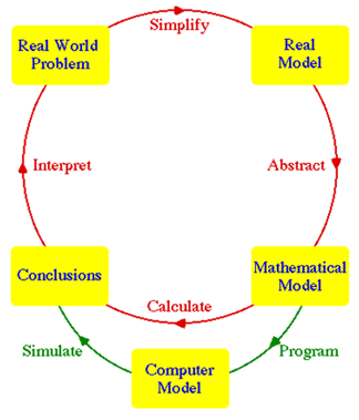
Mathematical modelling is a process by which a real - world problem can be described in the language of mathematics. The concept of modelling is used in all fields such as engineering, physics, chemistry, economics, computer science, biology etc. Banerjee (2021)

Figure 1

Figure 1  Scientific Process to Connect Real World Problem with Mathematics Source modelwithmathematics.com

       

The process of converting a real-world problem into a mathematical model involves several steps. First, the problem is identified and defined in the context of the real world. This problem is then translated into a mathematical model by formulating equations or formulas that represent the key aspects of the problem. The next step is to analyse the mathematical model to find some conclusions, often through solving these equations or using analytical methods to understand the system's behaviour. These mathematical conclusions are then implemented into a computer model, where computational techniques and software simulate the problem. The computer model generates predictions, which can be compared to actual observations or used to guide decision-making.

The application of mathematical models to solve problems in business or military operations is a core aspect of operational research. The defence budget represents the financial resources allocated by the state for the establishment and maintenance of armed forces or other defence-related activities. Defence expenditure includes all current and capital expenditure on the armed forces, including peacekeeping operations, expenditure by defence ministries and other government agencies involved in defence initiatives. It also includes paramilitary forces that are considered trained, equipped, and prepared for military operations.

The United States, China, Russia, India, Saudi Arabia, the United Kingdom, Germany, Ukraine, France, and Japan are often regarded as great powers due to their substantial military budgets. According to the Stockholm International Peace Research Institute, global military expenditure in 2021 reached $2,113 billion. Over the past 27 years, defence spending in both Russia and Ukraine have steadily increased in real terms.

The paper includes the classical Richardson-Arms race model and the modified Richardson-Arms race model with carrying capacity. These models are applied to defence spending data for Russia and Ukraine from 1994 to 2021.

 

 

2. Literature review

Moll and Luebbert (1980) reviewed covers 1970s quantitative studies on armament issues, categorized into Arms-Building Models and Arms-Using Models. It suggested that social and psychological factors are underrepresented in existing models, bureaucratic models are better predictors, and Arms-Using Models can assess military effectiveness but lack policy guidance. Future studies using recently developed empirical data show promise for rapid progress.

Schneider (1999) utilized five commonly applied models in defence spending studies. The aim was not to identify the single best model but to determine whether a consistent behavioural pattern could be observed across countries when using these models. They concluded that while the models do provide valuable insights into the defence spending behaviours of the two countries, they are not definitive and have limited applicability for forecasting purposes.

Dunne et al. (2003) analysed Richardson’s action-reaction model of arms races, which has inspired extensive empirical research. However, most efforts to estimate these models have proven unsuccessful. Leveraging recent advancements in time-series econometrics, they highlighted challenges in estimating such models for Greece and Turkey, as well as India and Pakistan. Their findings revealed minimal evidence of a Richardson-type arms race between Greece and Turkey, while India and Pakistan displayed a stable interaction characterized by a well-defined equilibrium.

Lehmann et al. (2009) modified the Richardson Arms Race Model by introducing a carrying capacity term to each equation, similar to the carrying capacity term in a logistic growth model. They found that introducing these terms allowed for the prediction of the level of armament for each country at the onset of war.

Chalikias and Skordoulis (2014) applied Lewis Richardson’s arms race model to analyse the advertising expenditures of two competitive firms in Greece's mobile phone industry, using secondary data. They concluded that the theoretical models align closely with real-world observations, suggesting that such models can be effectively applied to firms under suitable conditions.

Joseph et al. (2021) investigated the behaviours of a nation engaged in an arms race, aiming to understand the factors that could alter the course of the race. Their approach focused on the relationships between nations, allowing them to add and manipulate factors that directly affect the economic allocations a nation can make to fund its military production. They found that changes in a nation’s economy were consequences of its perceived expenditure, leading to a series of optimizations to maximize production.

Zhang and Chan (2021) demonstrated another potential application of Richardson’s Arms Race model beyond its original focus on defence and international conflicts. They applied the model to illustrate the competitive behaviour of two oligopolistic companies using R&D as a parameter.

 

3. Methodology

3.1. Classical Arms Race Model

Consider two neighbouring countries, A and B whose arms expenditures at time t are represented by x(t) and y(t) respectively in a standardized monetary unit. A simple mathematical model can be developed based on the principle of mutual fear: the more one country spends on arms, the more it motivates the other country to increase its own expenditure. Therefore, the rate of growth of each country's arms expenditure is directly proportional to the current expenditure of the other. Banerjee (2021) This relationship is mathematically expressed as:

 

 

where  and  are positive.

 

 

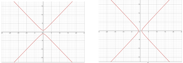
Figure 2

Figure 2 (a):                                                                    Figure 2 (b):

 

When , the graph implies that if nation  increases its arms expenditure, nation  will also increase or decrease but never cross the expenditure of . If  decreases its arms expenditure, then we have an increase or decrease in  but it always be more than the decrease of . When , we see the roles are reversed for both the cases above and hence similarly this is proved.

Equilibrium points

The equilibrium point is found by setting the right-hand side of equations equal to zero.

and

 

Thus, the equilibrium point is .

Here, we consider  for Russia and y for Ukraine, applying this model to their defence spending data from 1994 to 2021 on this model. We get the following values of constants,

 

,

 

Stability Analysis

To analyse the stability of the system around (0,0), we will consider the Jacobian matrix for the system. Letting   and  , the Jacobian matrix is

 

 

For our model, the Jacobian matrix is:

 

 

Substituting values of constants in this Jacobian matrix and matrix and evaluating at (0,0), we get

 

 

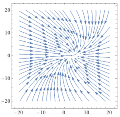
Computing the eigenvalues for the equilibrium point at (0,0) yields:

 

 

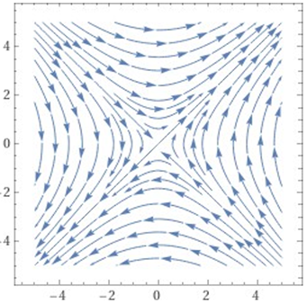
Here, one eigenvalue is positive and the other is negative. Therefore, the equilibrium point is unstable. Phase plane diagram also indicates that the equilibrium point is unstable.

Figure 3

Figure 3 Phase Plane Diagram

 

3.2. Richardson’s Arms Race Model

 

 

Thus,  as  and we conclude that both the countries A and B spend more and more money on arms with increasing time and no limits on the expenditure. As the mathematical prediction of indefinitely large expenditure for both the countries is unrealistic, an improved model is desired. Banerjee (2021)

We consider two neighboring countries A and B and let  and  be the expenditures on arms respectively by these two countries in some standardized monetary unit. A simplified refinement of model was made by Lewis F. Richardson (1881-1953), popularly known as the Richardson Arms Race model, where he assumed that each country spends on arms at a rate which is directly proportional to the existing expenditure of the other nation. Banerjee (2021)

He also assumed that the excessive expenditure on the arms puts the country’s economy in the compromising position and hence the rate of change of one country’s expenditure on arms will also be directly proportional to its own expenditure. He assumed that the cause of the increase of a country’s armament not only depend on mutual stimulation but also on the permanent underlying grievances of each country against the other. Banerjee (2021)

 

 

where are positive and  are constants which may have any sign.

Equilibrium points

The unique steady state solution is given by,

 

 

The equilibrium position exists if   .

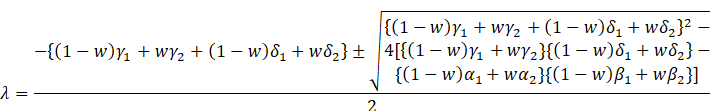
The characteristic equation is,

 

 

Let λ_1and  λ_2 be two roots of above characteristic equation.

 

 

Now, following four cases arises from it

Case 1

If

Then,  and

 

There is a position of equilibrium, and the system is stable. This means both the countries spent on arms in a strategic manner so that the economy of the country is not compromised.

Case 2 

If

Then

               

Thus, there is no position of equilibrium.

Also,

 &  are negative and expenditure cannot become negative.

In this case, to become negative they must pass through zero value.

As  becomes zero from, we get

 

 and

 

Thus,  decreases till it becomes zero.

Similarly, if  becomes zero from equation, we get  decrease till it reaches zero.

Thus, in this case there will ultimately be completely disarmament.

Case 3

If

These gives ,  

 

One of  , , is positive and other is negative.

In this case there will be a run – away arms race.

Case 4

If

These gives ,  

One of ,  is positive and other is negative.

In this case there will be a run-away arms race.

 

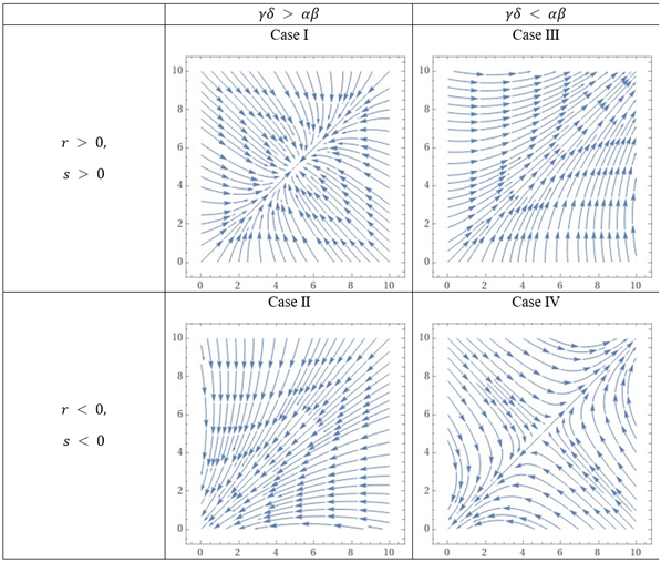
The shows four types of phase space diagrams indicating dynamics of the model according to relations among parameters .

Figure 4

Figure 4 Phase Plane Diagram

 

Here, we consider 𝑥 for Russia and 𝑦 for Ukraine and then apply to Russia and Ukraine defence spending data from 1994 to 2021 on this model. We get the following values of constants.

 

, , , , ,

 

Using the above values of constants the equilibrium point we get,

 

Stability Analysis

To analyse the stability of the system, we will consider the Jacobian matrix for the system. Letting  and , the Jacobian matrix is:

 

 

For our model, the Jacobian matrix is: 

 

 

Substituting values of constants in this Jacobian matrix and evaluating at (3.83,0.22), we have:

 

 

Computing the eigenvalues for the equilibrium point (3.83,0.22) yields:

 

 and

 

Here  and . Therefore, by stability theorem we conclude that equilibrium point is stable. Phase plane diagram also indicates that the equilibrium point is unstable.

Figure 5

Figure 5  Phase Plane Diagram

 

3.3. Modified Richardson’s Arms Race Model Involving carrying Capacity

Here, we all know very well that every country has limited amount of money to spent over arms and military. So, in this modification we add budget constrain   and . Here   is the maximum carrying capacity of expenditure on arms and military by country A and  is the maximum carrying capacity of expenditure on arms and military by country B.

Now, the modified Richardson’s arms race model can mathematically express as,

 

 

where  and r,s will be positive in case of mutual suspicions and negative in case of mutual goodwill.

Equilibrium points

The unique steady state solution is given by,

 

 

Here, there is a non-linear differential equation. So, we consider different cases obtaining equilibrium points. Here, we consider x for Russia and y for Ukraine and then apply to Russia and Ukraine defence spending data from 1994 to 2021 on this model. We get the following values of constants.

 

, , , , , , ,  

 

Case 1

 

 

So, in this case we can see that both countries have reached to their maximum carrying capacity of expenditure on arms and military. Using the values of constants the equilibrium point is,

 

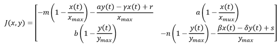
Stability Analysis

To analyse the stability of the system, we will consider the Jacobian matrix for the system. Letting  and , the Jacobian is:

 

 

For our model, the Jacobian is:

 

Substituting values of constants in this Jacobian matrix and evaluating at (88.35,44), we have:

 

 

Computing the eigenvalues for the equilibrium point (88.35,5.94) yields:

 

 

Here and . Therefore, by stability theorem we conclude that equilibrium point is stable.

 

Case 2

If

 

 

From above equations the steady state solution is establish only if  and satisfy above equation. Otherwise, arms race between them occurs. Using the above values of constants the equilibrium point is,

 

 

Stability Analysis

In order to analyze the stability of the system around (3.83,0.22), we will consider the Jacobian matrix for the system. Substituting values of constants in Jacobian matrix (case 1) and evaluating at (3.83,0.22), we have

 

 

Computing the eigenvalues for the equilibrium point (3.83,0.22) yields

 

 

Here and . Therefore, by stability theorem we conclude that equilibrium point is stable.

 

Case 3

 

From the above equation we can say that country A reaches its maximum carrying capacity, but country B may or may not reach its maximum carrying capacity. Using the above values of constants the equilibrium point is

 

 

Stability Analysis

To analyse the stability of the system around (88.35,0.24), we will consider the Jacobian matrix for the system. Substituting values of constants in Jacobian matrix (case 1) and evaluating at (88.35,0.24), we have

 

 

Computing the eigenvalues for the equilibrium point (88.35,0.24) yields

 

 

Here and . Therefore, by stability theorem we conclude that equilibrium point is stable.

 

Case 4

 

From the above equation we can say that country B reaches its maximum carrying capacity, but country A may or may not reaches its maximum carrying capacity. Using the above values of constants, the equilibrium point is,

 

 

Stability Analysis

To analyze the stability of the system around (7.03,5.94), we will consider the Jacobian matrix for the system. Substituting values of constants in Jacobian matrix (case I) and evaluating at (7.03,5.94), we have

 

 

Computing the eigenvalues for the equilibrium point (7.03,5.94) yields

 

 

Here  and . Therefore, by stability theorem we conclude that equilibrium point is stable.

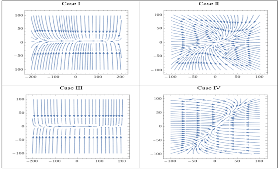
The following table shows phase space diagrams of each case.

Figure 6

Figure 6 Phase Plane Diagram

 

3.4. War scenario

If there is an ongoing war between two countries, and one country finds that its current military budget, based on last year's figures, is insufficient to sustain the conflict, it will need to significantly increase its military spending. In such a scenario, the concept of carrying capacity becomes irrelevant for that country due to the sudden surge in its military budget. Therefore, we need to modify our arms race model to account for this sudden increase in military expenditure. The proposed modification for this scenario is as follows:

consider two neighboring countries A and B with expenditures on arms represented by x(t) and y(t) respectively in a standardized monetary unit. During a war, if one country finds it impossible to sustain the conflict with its military budget based on the previous year, it will significantly increase its military budget to sustain the conflict. The modified arms race model can mathematically be expressed as,

 

 

Here , , are positive and  will be positive in case of mutual suspicions and negative in case of mutual goodwill. Also,  if there is no war and  if there is a situation of war.

Equilibrium points

The unique steady state solution is given by,

 

 

On solving above equations we get,

 

The equilibrium point/The steady state solution exists if  are positive.

Stability Analysis

To analyse the stability of the system, we will consider the Jacobian matrix for the system. Letting  and , the Jacobian matrix is:

 

 

For our model, the Jacobian matrix is:

 

 

And from the above Jacobian matrix we get eigen value as follow,

 

 

If all eigenvalues have negative real parts, the equilibrium point is stable otherwise the equilibrium point is unstable.

 

4. Conclusion

Our study delved into the classical arms race model and its application to the defence expenditures of Russia and Ukraine spanning from 1994 to 2021. Through stability analysis, we confirmed the stability of this model within the context of our dataset. Furthermore, we explored the Richardson arms race model, examining four distinct scenarios and illustrating them with phase plane diagrams. Introducing a carrying capacity component to the Richardson model, we identified and analyzed four stable equilibrium points. Additionally, by modifying Richardson’s Arms Race Model to simulate potential wartime conditions, we uncovered further insights into equilibrium points and their corresponding eigenvalues.

Our findings not only validate the applicability of arms race models in understanding defence spending dynamics between nations but also underscore the importance of incorporating nuanced factors such as carrying capacity and wartime scenarios. These insights contribute to the broader understanding of strategic decision-making in defence expenditures and provide a foundation for future studies in international relations and conflict resolution.

 

CONFLICT OF INTERESTS

None. 

 

ACKNOWLEDGMENTS

None.

 

REFERENCES

Alsabah, H., & Capponi, A. (2020). Pitfalls of Bitcoin's Proof-of-Work: R&D Arms Race and Mining Centralization. SSRN.

Banerjee, S. (2021). Mathematical Modelling: Models, Analysis and Applications. CRC Press. https://doi.org/10.1201/9781351022941

Bourgeois, L. (2024). Streaming Service Arms Race: Protection and Distribution of Live Sports Broadcasting in a Cord-Cutting Environment. Dalhousie Journal of Legal Studies, 33, 90.

Chalikias, M., & Skordoulis, M. (2014). Implementation of Richardson's Arms Race Model. Applied Mathematical Sciences, 8(81), 4013–4023. https://doi.org/10.12988/ams.2014.45336

Dunne, J. P., Nikolaidou, E., & Smith, R. (2003). Arms Race Models and Econometric Applications. In Arms Trade, Security and Conflict: Security and Conflict (pp. 178–198). Routledge. https://doi.org/10.4324/9780203477168.ch11

Hague, M. T., Stokes, A. N., Feldman, C. R., Brodie Jr, E. D., & Brodie III, E. D. (2020). The Geographic Mosaic of Arms Race Coevolution is Closely Matched to Prey Population Structure. Evolution Letters, 4(4), 317–332. https://doi.org/10.1002/evl3.184

Ishida, A. (2015). An Initial Condition Game of Richardson's Arms Race Model. Sociological Theory and Methods, 30(1), 37–50.

Joseph, R., Dhaliwal, M., & Basha, M. (2021). Arms Race Model.

Lehmann, B., McEwen, J., & Lane, B. (2009). Modifying the Richardson Arms Race Model with a Carrying Capacity.

Majeski, S. J., & Jones, D. L. (1981). Arms Race Modelling: Causality Analysis and Model Specification. Journal of Conflict Resolution, 25(2), 259–288. https://doi.org/10.1177/002200278102500203

Moll, K. D., & Luebbert, G. M. (1980). Arms Race and Military Expenditure Models: A Review. Journal of Conflict Resolution, 24(1), 153–185. https://doi.org/10.1177/002200278002400107

Roy, S., Mukherjee, A., Gautam, A., Bera, D., & Das, A. (2022). Chemical Arms Race: Occurrence of Chemical Defense and Growth Regulatory Phytochemical Gradients in Insect-Induced Foliar Galls. Proceedings of the National Academy of Sciences, India Section B: Biological Sciences, 92(2), 415–429. https://doi.org/10.1007/s40011-021-01322-2

Sadeghi, K., Banerjee, A., & Gupta, S. K. (2020). A System-Driven Taxonomy of Attacks and Defenses in Adversarial Machine Learning. IEEE Transactions on Emerging Topics in Computational Intelligence, 4(4), 450–467. https://doi.org/10.1109/TETCI.2020.296893

Schneider, J. W. (1999). What drives defence spending in South Asia? An Application of Defence Spending and Arms Race Models to India and Pakistan (Doctoral dissertation, Virginia Tech).

Zhang, K., & Chan, Z. Q. (2021). Application of Richardson's Arms Race Model in Oligopolistic Competition. International Journal of Science and Research (IJSR). https://doi.org/10.21275/SR21122184103