COMPUTATIONAL PERFORMANCE OF HOLE FILLING MORPHOLOGICAL ALGORITHMS FOR BINARY IMAGES

 

Gonzalo Urcid ¹, José-Angel Nieves-Vázquez ², Rocío Morales-Salgado ³

 

¹ Ph.D., Optics Department, INAOE, Tonantzintla 72840, Mexico

² Ph.D., Engineering Division, ITSSAT, Matacapan 95804, Mexico

³ Ph.D., Information and Data Science Department, UPAEP, Puebla 72410, Mexico

 

1. INTRODUCTION

The subject of morphological binary image processing Serra (1986), Maragos (1987), Haralick et al. (1987), Dougherty (1992) is a branch of the more general subject of digital image processing and analysis. Binary image processing deals with black and white digital images whose values are coded with 0’s and 1’s, where the zero ‘0’ and one ‘1’ values are commonly interpreted, respectively, as background and foreground pixels. The foreground pixels may form one or more white shapes or regions in the image that usually correspond to objects of interest surrounded by a black background Pitas (2000), Gonzalez & Woods (2018). Since binary images are a special case of gray scale images, it turns out that for “looking” or “displaying” a binary image coded with 0’s and 1’s, it is mapped to the gray scale dynamic range of non-negative integer values belonging to [0,255] assuming that the grayscale image is coded with 8 bits per pixel. Hence, for displaying purposes, the minimum value ‘0’ still represents black and the maximum value ‘255’ corresponds to white. Image processing tasks such as object segmentation and object recognition may produce a binary image that is obtained from thresholding or quantizing a grayscale image Pitas (2000), Najman & Talbot (2010), Gonzalez & Woods (2018), Gonzalez et al. (2020). The output binary image then requires some kind of post-processing to prepare it for further analysis. A typical situation is the presence of holes, cracks, or scratches in several regions of a binary image that need to be removed by filling them. For example, possible reasons for the presence of holes in a binary image is due to occluding objects, low reflectance subregions, or missing scanned portions ocurring in grayscale images. We remark that using the corresponding digital topology associated with an underlying digital grid such as the square grid, holes, cracks, and scratches can be considered as the same type of image artifact. Henceforth, we will use the word “hole” to represent any of the previously mentioned items. From a geometrical point of view, based on set theory, mathematical morphology has devised simple and effective hole filling algorithms to tackle the aforementioned problem as can be seen in Vincent (1992), Vincent (1993), Géraud et al. (2010) . In this research paper, we present a computational performance analysis of the fundamental region filling procedures based on mathematical set morphology.

Recent contributions with respect to the basic hole filling morphological algorithms are described in Hasan & Mishra (2012), Valdiviezo et al. (2017). The work presented in Hasan & Mishra (2012) suggests the use of a different initial marker image for increasing the number of seed points used in the dilation operation as well as the dynamic use of two structuring elements, the “diamond” and “square” structuring elements of size , combined with thresholding for corrections of local 4-connectivity and 1-pixel-thin border object processing. On the other hand in Valdiviezo et al. (2017), a supervised hole filling algorithm based on morphological conditional dilation is based on chosing a single background pixel as the marker image and has the advantage of being very simple. However, this last scheme although interactive in nature, happens to be a particular case of the more general mechanism explained in Subsection 3.2 for the unsupervised algorithm. Also, alternative advances that realize improvements over the hole filling morphological algorithms are described in Fanfeng & Wei (2010), He et al. (2019). However, we do not delve into these last works since their computer implementation requires additional non-morphological techniques that would require other performance measures besides the number of iterations that we have selected for our computational tests.

Our paper is organized as follows: in Section 2 we will give only the necessary mathematical morphology operations involved in hole filling algorithms. However, for the interested reader, in depth treatments of the basic morphological operations including additional ones derived using dilation and erosion, their algorithmic implementation as well as their applications to other tasks in digital image processing and analysis can be found in Rivest et al. (1993), Van Droogenbroeck (1994), Bloch et al. (2007), Beucher & Beucher (2012), Gonzalez & Woods (2018) and Gonzalez et al. (2020). Section 3 gives in detail the theoretical description of the fundamental mathematical morphology hole filling techniques emphasizing the central role of the marker image and henceforth, classifying the corresponding computational procedures as supervised or unsupervised. In Section 4, we present our tests on various representative binary digital images using as a measure of computational performance, the number of iterations needed in each algorithm as applied to each binary image to produce the desired result. We end our paper with Section 5 to expose the conclusions of this research work as well as some pertinent comments on future developments.

 

2. BACKGROUND ON MATHEMATICAL MORPHOLOGY

Mathematical morphology as applied to digital image processing is a mathematical theory that is concerned with analysing and extracting form or shape information from objects contained in a given image. The basic scenario does occur in binary images where the notions of foreground objects and background are in general clearly distinguished in the context of specific real-world applications. Two encodings are possible in binary image processing, i. e., white foreground (WF) objects immersed in a black background (BB), denoted for short as WF-BB, or black foreground (BF) objects embedded in a white background (WB) abbreviated as BF-WB. Algebraically speaking, both encodings, WF-BB and BF-WB, are dual to each other using binary complementation. Here we will use the first encoding. Note that the WF-BB coding is a particular case of grayscale 8-bit encoding whose dynamic range of 256 values is reduced from the non-negative integer interval, , to the two-value set . On the other hand, the BF-WB encoding is generally employed in silhouette, artistic binary image processing or in theoretical descriptions based on graph theory. In this paper, only square images of size  picture elements are used to simplify symbolic expressions in mathematical arguments and also since the extension to rectangular images is rather trivial.

 

2.1. Operations on Sets, Dilation and Erosion

We assume the reader is familiar with set relations such as inclusion and equality as well as the set operations of union, intersection, difference, and complementation. Some geometrical operations on sets follow. If , with origin , represents the two-dimensional digital space, let , then the complement A is defined as , and the symmetrical, origin reflected or transpose of A is considered to be the set . Also, if , the translation of A by x, or translate  is the subset of S specified by . In order to extract shape information from objects contained in a given image, the basic mechanism from the stand point of mathematical morphology, is to use a geometrically well-defined tiny shape as a probe that scans and interacts pixelwise with foreground objects and background. The elementary morphological operations, known as dilation and erosion, work with these tiny shapes formally called structuring elements, respectively to grow or shrink image objects. Thus, given a binary image A and a structuring element B, both considered as subsets of S, dilation and erosion of image set A by structuring element B are defined, respectively, by the left and right expressions in (1),         

 

 

where x denotes locations or points in digital space S and  and  denotes the translate of the symmetric structuring element, respectively, itself, to location . Note that dilation of A by B, denoted as , is a new set formed by all points  such that  displaced at each x, overlaps or hits at least some portion of A. Analogously, erosion of A by B, in symbolic terms , refers to a new set consisting of all points  such that B translated by x fits completely within A. The second equality shown in the left and right expressions in (1) are the equivalent set-theoretical operations corresponding to Minkowski addition and Hadwiger substraction, which make clear, the upsizing or downsizing nature of A by B through a generalized union or intersection of translates. We point out that dilation and erosion are dual by complementation in the sense that dilating set A with structuring element B is equivalent to perform and erosion of its complement with the symmetrical of  as established in (2),

 

 

Qualitatively, dilation enlarges an object, changes its convex corners, and reduces its surrounding background. Similarly, erosion reduces an object, changes its concave corners, and enlarges its neighbouring background. In relation to the morphological region filling algorithms exposed in Section 3, we will use only the dilation operation together with set complementation. Particularly, if B is a structuring element the repeated dilation of B with itself, i. e.,  is written as 2B. In addition, if A is a single element set, i. e., , then from (1) it follows readily that,

 

     

 

meaning that dilation of a single (isolated) point x by B is equivalent to a geometrical translation of B to x which is coincident with B’s origin. Also, erosion of a single point x by B has the effect of removing the point since B displaced to x is not a subset of {x}.  A structuring element will be abbreviated as SE. More specifically, use is made of 3×3 SE’s having 4-connectivity (straight cross ‘+’ or diagonal cross ‘×’), and 8-connectivity (square block ‘■’).                                                                                                                 

 

2.2. Image Border, Holes and Local Knowledge

For a binary image  of size  pixels, the border or frame of A, denoted by , is defined by the set of pixels given by the union of the top (first) and bottom (last) rows of pixels together with the left (first) and right (last) columns of pixels. Thus, , where , , , , and  for all i and j. A hole is defined as a background region in which any pixel is surrounded by a connected path of foreground pixels. An alternative definition of a hole is a background region that is bounded by a foreground object. Equivalently, no connected path of background pixels exists between any pixel in a hole and a background pixel of . It should be clear that the border of an image not only delimits its size but also its contents. Hence, a physical sensor of finite dimensions that acquires or captures an image from a real scene will provide us with partial or local knowledge relative to objects or foreground regions contained in the original scene. In the case of objects with holes,  may cut or truncate portions of their corresponding regions leaving them “unfinished” or “incomplete” beyond the image frame. Therefore, in a strict sense, truncated holes, cracks or scratches cannot be considered as such due to incomplete knowledge outside the image border. However, the ocurrences just mentioned may be filled or not depending of contextual image content and its interpretation for further processing.

 

3. MORPHOLOGICAL REGION FILLING ALGORITHMS

The hole filling algorithms based on mathematical morphology can be categorized as supervised or unsupervised, and each one of them is founded on specific morphological set operations between the image itself and an auxiliary image known as the marker image, which in turn is derived from the given input image. The algorithms have been devised to be iterative in nature and therefore convergence to the desired result, i. e., the filled image is guaranteed to be obtained in a finite number of steps.

 

3.1. Supervised Filling Algorithm

A mathematical morphology hole filling algorithm is said to be supervised if the marker image is derived from the input image by selecting interactively an adequate subset of pixels. The chosen pixels may belong to image oject regions, to the image background or a mixture of both. Assuming that m holes  for  exist in one or more objects as foreground regions in a given binary image A of size , the common choice, as exposed in preliminary treatments on mathematical morphology of sets and its applications to binary images Gonzalez & Woods (2018), Gonzalez et al. (2020) consists in taking a single point or pixel  belonging to each hole . Thus, the marker image M or set of markers is defined as the set , where  is not a proper subset of A and . The basic morphological hole filling algorithm consists of an iterative scheme based on conditional dilation as specified in the following equation:

 

 

where,  is a symmetric structuring element corresponding to  elementary neighborhood with 4 (straight or diagonal cross), 6 (hexagon) or 8 (square) connectivity, and  is the complement of A. Computation of  is repeated until  and the final iteration stops at  . In the last step, the union set  contains the original object regions with their holes, cracks, or scratches filled. Note that, in (4), the intersection of  at each iteration with  limits the expanding effect of performing successive dilations. To cover every aspect, we explain in more detail how the basic algorithm works. Specifically, we can write the marker set as , where each point  and  is a subset corresponding to a hole within an object region that properly may have more than one hole and which we write as . We also assume that the structuring element contains the origin, thus . Unfolding the iterative conditional dilation for  we have that

 

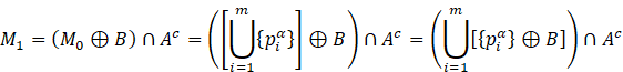
where  is the structuring element translated to point  after applying the first expression in (3), and  for any i. Similarly, for , we obtain,

 

 

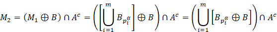
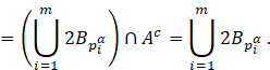
Note that,  can be written as  since dilation at each iteration is performed on the previously grown set  . Thus, the result of the l-th iteration is given by  , where . At this stage, several points in  have been expanded to their corresponding hole sizes and the remaining unfilled holes still require further iterations until the growing scheme stops after masking once more with . Therefore, for , it happens that  which in turn implies that , and the resulting set,  contains the required flooded holes. Finally, set  gives the desired result by gluing all the filled holes with the original image. Consequently, all multiconnected foreground regions or equivalently objects with one or more holes are changed to simple connected regions, i. e., objects without holes, cracks or scratches. The supervised morphological filling algorithm will be abbreviated as SMFA.

 

3.2. Unsupervised Filling Algorithm

A mathematical morphology hole filling algorithm is said to be unsupervised if the marker image is derived from the input image by means of a mathematical function or by an automatic procedure that defines an adequate proper subset of pixels (cf., e.g., Hasan & Mishra (2012) and Gonzalez & Woods (2018)). Again, selected image points may be background, foreground or a combination of both types of pixels. In the present context used is made of what is known as morphological reconstruction and the terminology is changed to convey its generality upon application of more advanced morphological mathematical operations such as opening or closing which fall outside the scope of this work. Specifically, morphological conditional dilation turns to be morphological geodesical dilation, the input or source image is consider as a mask to control geodesical dilation growth or reconstruction, and the role of the marker image is the same as previously explained, except that it is defined by a mathematical function as already mentioned above. For the case at hand, the marker image M corresponding to the mask image usually denoted by G is given by,

 

 

Interpretation of (5) in terms of image content is that, , a set difference equal to the void set gives us a full black background image of which we change the image border, i.e.,  with white pixels all around except where foreground objects touch it and become black pixels. If  denote the integer spatial coordinates of image G (the mask or input image), where , then the matrix expression associated with (5) is the following:

 

 

Worth to remark is the fact that the marker image M as established in (6) is a set of pixels with a special structure that is not a subset of G. In particular, if  is a background pixel then , meaning that the selected image border pixel is turned “on”, i. e., becomes a marker. In case  is a foreground pixel then , hence the corresponding image border pixel is turned “off” or equivalently is not consider a marker point. Thus, M contains only background pixels as marker points. As mentioned earlier, in morphological processing several image manipulations are derived from a parametric operation known as morphological recontruction that considers two images, the marker image M and the mask image G together with a symmetric structuring element B which is a  elementary neighborhood with 4, 6 or 8 connectivity. Notice that in general G is not necessarily equal to a given input image A. Furthermore, in the case of filling one or more holes using (6) it turns out that . Particularly, the morphological geodesic dilation of size n is defined recursively as,

 

                                                                                 

 

expression interpreted as the morphological geodesic dilation of size 1. Recalling the way M is defined, the unsupervised hole filling algorithm using morphological geodesic dilation is based on the following iterative procedure,

 

 

until stability is accomplished, i. e., when  and  is the last iteration. In the final step, the output or final image  with all holes filled is determined by computing,

 

              

 

Again, for the sake of completeness, we present how the algorithm given by (8) and (9) works. As before, we can write the marker set as , where each point , , and  is the subset corresponding to the image border. Note that M does not contain any point marking a hole within an object region. Recalling that the structuring element contains the origin, i. e.,  and that the mask , the morphological geodesic dilation for  is given by

 

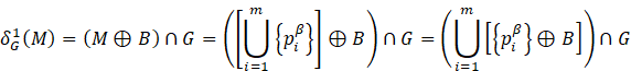
where  is the structuring element translated to point  after applying the first expression in (3), and  for any i. Similarly, the morphological geodesic dilation for , results in,

 

 

In similar fashion, the result of the l-th iteration is given by  , where . At this stage, all points in M have been expanded within the mask G covering almost all space outside the exterior edges of object regions with or without holes, no matter their number or size. Further iterations fills up the remaining external space and dilation stops after masking once more with G and obtaining a result equal to the previous one. Therefore, for , it happens that  which in turn implies that , and the resulting set,  contains the flooded space that surrounds the exterior edges of all object regions. Finally, set  gives the desired result since the complement of the external space between all object regions contains all original foreground regions including those with filled holes. In this case, the set difference,  gives an image with all filled holes, cracks, or scratches. The unsupervised morphological filling algorithm will be abbreviated as UMFA.

 

3.3. Algorithm Comparison

From the discussion presented in Subsections 3.1 and 3.2, it can be seen that the supervised and unsupervised versions of the morphological hole filling algorithm share the same structural iterative procedure to attain their goal. However, as has been explained in detail, their main difference resides in the way the marker image is established, which in turn distinguishes their mode of operation, that is, interactive versus automatic, hence the use of a superscript for marker points within holes versus the use of the β superscript for marker points belonging to the image border.

In supervised mode we made the assumption that the number of holes is much less than the number of pixels in a given square image, i. e. , which in turn is related to the number of connected or multiconnected object regions. In unsupervised mode, the number of seed points or initial markers is bounded by the number of pixels on the image border, i. e. , and is derived from the manner in which the marker image is defined by means of a mathematical function. It is not difficult to see that the variables n and m are essential to determine the computational complexity of each algorithm. However, to date there is no explicit functional expression for the corresponding computational complexity for parallel and sequential implementations of both algorithms (cf. Sec. IV in Vincent (1993) ). Nonetheless, computational tests can be based on measuring execution time or counting the number of iterations to achieve the desired result. Execution time is dependent on computing machinery characteristics and iteration count depends on programming implementation either parallel or sequential. Specifically, we will use the iteration count criterion to compare our implementation of the morphological filling algorithms previously described.

 

4. COMPUTATIONAL TESTS ON BINARY IMAGES

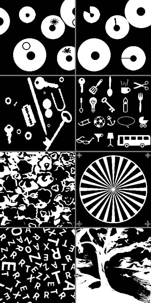
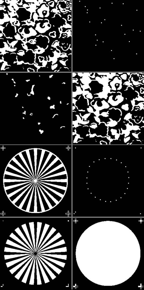
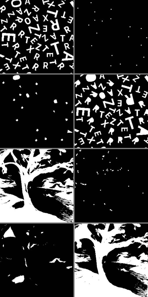
The results obtained with a computer implementation of the supervised and unsupervised morphological hole filling algorithms using the Mathcad high level programming language are presented in detail. In comparing both techniques, 15 binary images of size 256×256 pixels with WF-BB encoding were used. However, to ilustrate visually the results obtained, 8 digital binary images were selected as displayed in Figure 1. A description of all test images is listed in Table 1 where selected images for display are marked on the right with an asterisk (*).

Table 1

Table 1 Set of 16 Test Binary Images used for Morphological Hole Filling
Test Image	Holes	Description
‘00’	2	two-hole small image 32×32 px (initial testing)
‘01’	1	single hole within a disk
‘02’	14	multiple round holes
‘03’	15	multiple irregular holes
‘04’	6	multiple holes of different shapes *
‘05’	3	holes and scracthes *
‘06’	10	set of simple tools, several shapes *
‘07’	34	several simple object silhouettes *
‘08’	13	multiple holes within particles
‘09’	23	multiple holes within irregular particles *
‘10’	43	multiple small holes within cells
‘11’	29	multiple sector holes in a circular pattern *
‘12’	30	holes in letters of a sample text
‘13’	20	holes in letters of unequal size & orientation *
‘14’	57	multiple sized holes within a natural scene *
‘15’	6	holes within an artificial object composition

 

In the following pages, the results obtained with the supervised morphological filling algorithm (SMFA) are shown in Figure 2, Figure 3, Figure 4, Figure 5. Next, the results obtained with the unsupervised morphological filling algorithm (UMFA) are given in Figure 6, Figure 7, Figure 8, Figure 9. In both groups of results the structuring element used was the straight cross ‘+’ of size 3×3 pixels whose corners are turned ‘off’ (0) and any other pixel is ‘on’ (255). For visualization purposes points within holes, serving as markers, are displayed as white boxes of size 3×3 pxs and clearly, only the center point is employed for operating with the SMFA. Similarly, background points on the image border  used as markers have been dilated to a 3×3 pixel size and shown in red color to emphasize their nature. Again, only single pixels belonging to the image border are used to operate the UMFA. The numerical values of the iteration count for each test binary image using both algorithms with SE’s, ‘+’ (4-connectivity) and ‘■’ (8-connectivity) are listed in Table 2 that appears after Figure 9.

 Figure 1

Figure 1 1st Group of 8 Sample Binary Images Selected from a set of 15 Test Images. Label Numbers from Left to Right, Top to Bottom is ‘04’, ‘05’, ‘06’, ‘07’, ‘09’, ‘11’, ‘13’, ‘14’ and Separation Between Images is Shown in Gray.

Figure 2

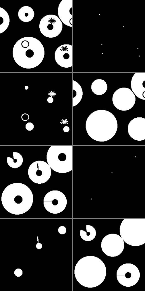
Figure 2 Results for Binary Images ‘04’ and ‘05’ using SMFA and SE=‘+’. For Image ‘04’, 1st Row: Left, Source Image; Right, Marker Image with 6 Points (Holes). 2nd Row: Left, Filled Holes; Right, Source Image with Holes Filled. For Image ‘05’, 3rd and 4th Rows: Same Clockwise Sequence as in Previous Binary Image. Marker Image has 3 Points (Holes).

Figure 3

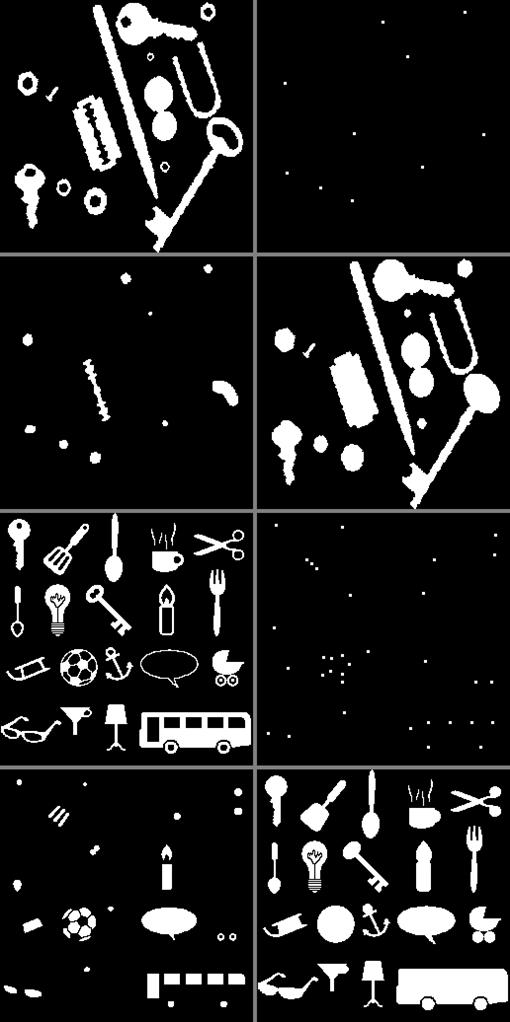
Figure 3 Results for Binary Images ‘06’ and ‘07’ using SMFA and SE=‘+’. For Image ‘06’, 1st Row: Left, Source Image; Right, Marker Image with 10 Points (Holes). 2nd Row: Left, Filled Holes; Right, Source Image with Holes Filled. For Image ‘07’, 3rd and 4th Rows: Same Clockwise Sequence as in Previous Binary Image. Marker Image has 34 Points (Holes).

Figure 4

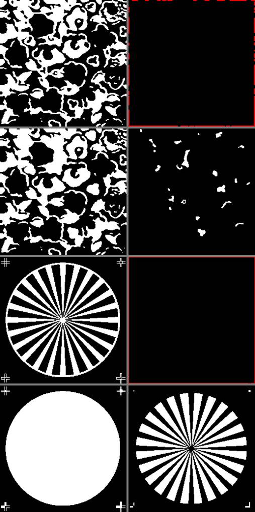
Figure 4 Results for Binary Images ‘09’ and ‘11’ Using SMFA and SE=‘+’. For Image ‘09’, 1st Row: Left, Source Image; Right, Marker Image with 23 Points (Holes). 2nd Row: Left, Filled Holes; Right, Source Image with Holes Filled. For Image ‘11’, 3rd and 4th Rows: Same Clockwise Sequence as in Previous Binary Image. Marker Image has 29 Points (Holes).

Figure 5

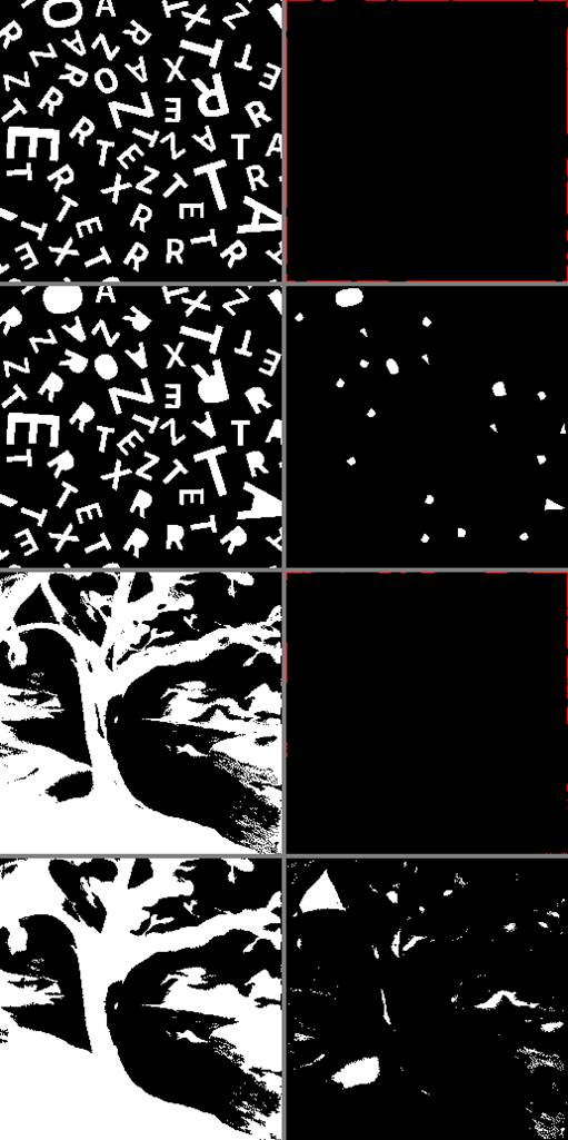
Figure 5 Results for Binary Images ‘13’ and ‘14’ Using SMFA and SE=‘+’. For Image ‘13’, 1st Row: Left, Source Image; Right, Marker Image with 20 Points (Holes). 2nd Row: Left, Filled Holes; Right, Source Image with Holes Filled. For Image ‘14’, 3rd and 4th Rows: Same Clockwise Sequence as in Previous Binary Image. Marker Image has 57 Points (Holes).

Figure 6

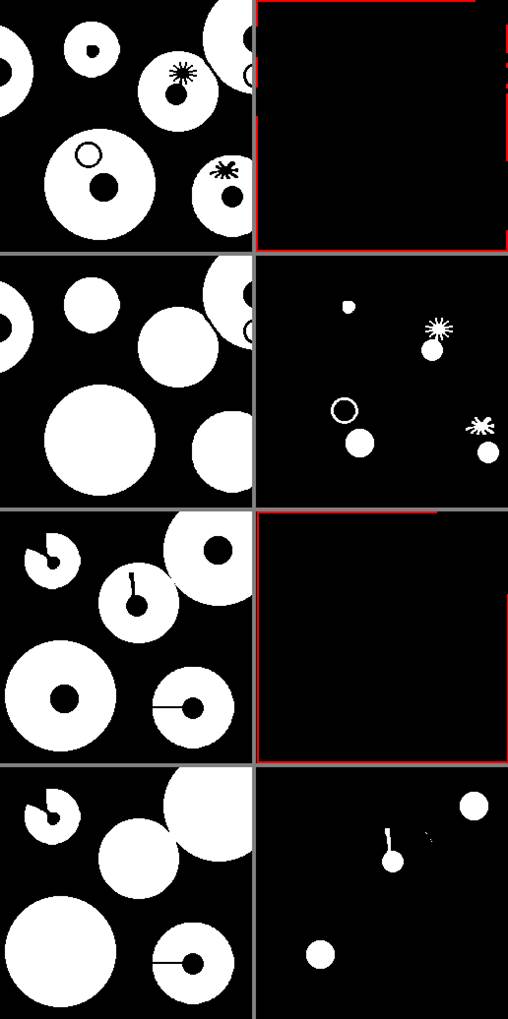
Figure 6 Results for Binary Images ‘04’ and ‘05’ Using UMFA and SE=‘+’. For Image ‘04’, 1st Row: Left, Source Image; Right, Marker Image with Border Points (Red Color). 2nd Row: Left, Source Image with Holes Filled; Right, Filled Holes. For Image ‘05’, 3rd and 4th Rows: Same Clockwise Sequence as in Previous Binary Image. Marker Image Shows Border Points in Red.

Figure 7

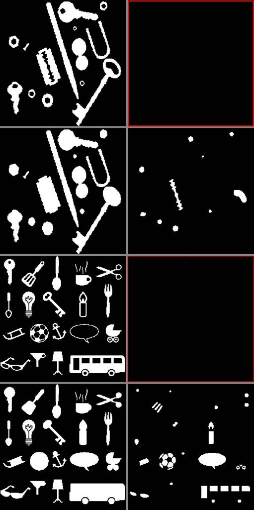
Figure 7 Results for Binary Images ‘06’ and ‘07’ Using UMFA and SE=‘+’. For Image ‘06’, 1st Row: Left, Source Image; Right, Marker Image with Border Points (Red Color). 2nd Row: Left, Source Image with Holes Filled; Right, Filled Holes. For Image ‘07’, 3rd and 4th Rows: Same Clockwise Sequence as in Previous Binary Image. Marker Image Shows Border Points in Red.

Figure 8

Figure 8 Results for Binary Images ‘09’ and ‘11’ Using UMFA and SE=‘+’. For Image ‘09’, 1st Row: Left, Source Image; Right, Marker Image with Border Points (Red Color). 2nd Row: Left, Source Image with Holes Filled; Right, Filled Holes. For Image ‘11’, 3rd and 4th Rows: Same Clockwise Sequence as in Previous Binary Image. Marker Image Shows Border Points in Red.

Figure 9

Figure 9 Results for Binary Images ‘13’ and ‘14’ using UMFA and SE=‘+’. For Image ‘13’, 1st Row: Left, Source Image; Right, Marker Image with Border Points (Red Color). 2nd Row: Left, Source Image with Holes Filled; Right, Filled Holes. For Image ‘14’, 3rd and 4th Rows: Same Clockwise Sequence as in Previous Binary Image. Marker Image Shows Border Points in Red.

Table 2

Table 2 Count Iteration k for Each Test Binary Image Using Morphological Hole Filling
Test Image	Holes	SMFA ‘+’	SMFA ‘■’	UMFA ‘+’	UMFA ‘■’
‘00’	2	9	7	13	13
‘01’	1	50	34	103	103
‘02’	14	12	9	287	255
‘03’	15	20	16	303	245
‘04’	6	49	33	261	255
‘05’	3	41	34	249	249
‘06’	10	43	32	315	255
‘07’	34	35	202 §	273	255
‘08’	13	23	17	331	233
‘09’	23	36	340 §	461	329
‘10’	43	10	138 §	285	255
‘11’	29	111	75	91	91
‘12’	30	5	4	263	255
‘13’	20	19	13	301	257
‘14’	57	59	133	757	291
‘15’	6	330	305	255	243

 

Comparing the iteration count in Table 2 between the 3^rd and 5^th columns one can see that the k values obtained with the SMFA ‘+’ are less than those obtained by applying the UMFA ‘+’, except for test images ‘11’ and ‘15’. A similar comparison occurs between the 4^th and 6^th columns, where k values are greater for the UFMA ‘■’ than for the SFMA ‘■’, except for test images ‘09’ and ‘15’. In general, the number of iterations required by the SFMA is much less than the number needed by the UFMA. The difference, as explained earlier, lies in the manner the marker images are built, i. e., interactively versus autonomously. However, the greater advantage of morphological recontruction from border points against conditional dilation based on seed points within holes is that, the first one as an automatic procedure does not require user intervention. Standard actual computer equipment spends milliseconds even for greater values of k such as those obtained with the UFMA and is independent of the number of holes. In disadvantage, minutes are consumed, before applying the SFMA, in preparing a marker image that depends on the number of holes and their spatial location.

An important remark is in order. In column 4, the k value for test images ‘07’,’09’ and ‘10’ has the symbol ‘§’ meaning that “locally” there are pixels which are 8-connected to the background and therefore the use of the box ‘■’ as SE, does not work correctly in treating single pixels as part of a hole. Hence, although convergence is reached, the image results fail to be useful. Finally, as a rule of thumb, both SFMA ‘+’ and UFMA ‘+’ can be used securely in practical applications, the second being the best due to its conceptual characteristics.

 

5. CONCLUSIONS

In this paper, the computational performance between supervised and unsupervised morphological hole filling algorithms has been analysed mathematically using explicit and detailed arguments based on set mathematical morphology. In addition, a representative collection of binary test images were used for showing qualitatively image results obtained by running both type of algorithms as well as quantitative numerical results obtained by keeping track of the total number of iterations required for convergence. Future work contemplates, for example, the study of possible correlations between the number of holes and the number of iterations needed.

 

CONFLICT OF INTERESTS

None. 

 

ACKNOWLEDGMENTS

Gonzalo Urcid thanks the National System of Researchers (SNII-CONAHCYT) in Mexico City for partial financial support through grant No. 22036. José-Angel Nieves-V. thanks TecNM campus San Andrés Tuxtla for partial financial support during the development of the present research and Rocío Morales-S. is grateful to UPAEP for taking work time to participate in this research project.

 

REFERENCES

Beucher, N. & Beucher, S. (2012). Mamba: Mathematical Morphology Library Image for Python Programming Language.

Bloch, I., Heijmans, H., & Ronse, C. (2007). Mathematical Morphology. In M. Aiello, I. Pratt-Hartmann, & J. Van Benthem (Eds.), Handbook of Spatial Logic. (Ch. 14, 857-875). Springer.

Dougherty, E. R. (1992). An Introduction to Morphological Image Processing. SPIE Tutotial Texts in Optical Engineering, Bellingham, Washington, USA, 9, 39-42.

Fanfeng, Z. & Wei, F. (2010). Hole Filling Algorithm Based on Contours Information. In Proceedings of 2nd International Conference on Information Science and Engineering, Hangzhou, China. IEEE Xplore, https://doi.org/10.1109/ICISE.2010.5691941

Gonzalez, R.C. & Woods R.E. (2018). Morphological Image Processing. In Digital Image Processing, 4th Global ed.  (Ch. 9, 653-655 & 667-674). Pearson, New York, NY, USA.

Gonzalez, R.C., Woods, R.E., & Eddins S.L. (2020). Morphological Image Processing. In Digital Image Processing Using MATLAB, 3rd ed. (Ch. 10, 614-618). Gatesmark Publishing.

Géraud, T., Talbot, H., & Van Droogenbroeck, M. (2010). Algorithms for Mathematical Morphology. In L. Najman & H. Talbot (Eds.), Mathematical Morphology: From Theory to Application. (Ch.12, 323-352). ISTE/Wiley & Sons, UK/USA. https://doi.org/10.1002/9781118600788.ch12

Haralick, R.M., Sternberg, S.R., & Zhuang X. (1987). Image Analysis Using Mathematical morphology. IEEE Trans. on Pattern Analysis and Machine Intelligence, PAMI-9(4), 532-550, https://doi.org/10.1109/TPAMI.1987.4767941 

Hasan, M.M. & Mishra, P.K. (2012). Improving Morphology Operation for 2D Hole Filling Algorithm. International Journal of Image Processing (IJIP), 6(1), 1-12.  

He, Y., Hu, T., & Zeng, D. (2019). Scan-Flood Fill (SCAFF): An Efficient Automatic Precise Region Filling Algorithm for Complicated Regions, 761-769. 2019 IEEE/CVF Conference on Computer Vision and Pattern Recognition Workshops (CVPRW), Long Beach, CA, USA. IEEE Xplore, https://doi.org/10.1109/CVPRW.2019.00104

Maragos, P. (1987). Tutorial on Andvances in Mophological Image Processing and analysis. Optical Engineering, 26(7), 623-632, https://doi.org/10.1117/12.7974127

Najman, L. & Talbot, H. (2010). Introduction to Mathematical Morphology. In L. Najman and H. Talbot (Eds.), Mathematical Morphology: From Theory to Application. (Ch. 1, 3-33). ISTE/Wiley, Great Britain/USA, https://doi.org/10.1002/9781118600788.ch1

Pitas, I. (2000). Shape Description. In Digital Image Processing Algorithms and Applications, 361-369. John Wiley & Sons, New York, USA.

Rivest, J-F., Soille P., & Beucher S. (1993). Morphological Gradients. Journal of Electronic Imaging, 2(4), 326-336. https:/doi.org/10.1117/12.159642.   

Serra, J. (1986). Introduction to Mathematical Morphology. Computer Vision, Graphics, and Image Processing, 35, 283-305, https://doi.org/10.1016/0734-189X(86)90002-2

Soille, P. (2004). Geodesic Transformations. In Morphological Image Analysis: Principles and Aplications, 2nd ed. (Ch. 6, 183-216). Springer-Verlag, Berlin-Heidelberg, Germany. 

Valdiviezo-N., J.C., Urcid, G., & Edwin, L. (2017). Digital Restoration of Damaged Color Documents Based on Hyperspectral Imaging and Lattice Associative Memories. Signal, Image and Video Processing (SIViP), 11, 937-944. https://doi.org/10.1007/s11760-016-1042-y

Van Droogenbroeck, M. (1994). On the Implementation of Morphological Operations. In J. Serra & P. Soille (Eds.), Mathematical Morphology and Its Applications to Image Processing, 241-248. Kluwer Academics, The Netherlands.  

Vincent, L. (1992). Morphological Algorithms. In E.R. Dougherty (Ed.), Mathematical Morphology in Image Processing, 255-288. CRC-Press, Boca Raton, FL, USA.  https://doi.org/10.1201/9781482277234   

Vincent, L. (1993). Morphological Grayscale Reconstruction in Image Analysis: Applications and Efficient Algorithms.  IEEE Transactions on Image Processing, 2(2), 176-201. https://doi.org/10.1109/83.217222