EXAMINING THE IMPACT OF DEBT MATURITY TIME, EXPECTED RETURN AND VOLATILITY ON PROBABILITY OF DEFAULT IN CREDIT RISK MODELLING: THE CASE OF MERTON AND MKMV MODELS

 

George Jumbe ¹, Ravi Gor ²

 

¹ Research Scholar, Department of Mathematics, Gujarat University, India

² Department of Mathematics, Gujarat University, India

 

1. INTRODUCTION

Default risk, also known as default probability, is the likelihood that a borrower won't pay back the principal and interest owed on a debt security in whole and on time. One of the two elements of credit risk is default risk, along with loss severity. The chance of a default over a specific time horizon is described by the financial risk management term probability of default (PD). It offers a prediction of the probability that a borrower won't be able to pay back its debt. The PD is normally determined by performing a migration study of loans with similar ratings over a certain time period and calculating the proportion of defaulted loans. The PD is then assigned to the risk level and each risk level will only have one PD percentage Joseph (2021).

The PD can be used in a wide range of different credit analysis or risk management scenarios. It is influenced by the borrower's qualities as well as the overall state of the economy. In order to make up for the increased default risk, creditors (lenders) often demand a higher interest rate. Various credit evaluations and risk management frameworks make use of the PD especially in the determination of the economic or regulatory capital for a banking organization.

The PD is closely related to the expected loss, which is calculated as the sum of the Product Derivative (PD), Loss Given Default (LGD), and Exposure at Default (EAD). This study explore the effects of volatility, expected return, and debt maturity time on probability of default in credit risk using Merton and Moody's KMV model.

 

2. LITERATURE

Peresetsky et al. (2011) conducted an econometric analysis of Russian bank failures from 1997 to 2003, concentrating on the degree to which information from quarterly bank balance sheets that is made publicly available can be used to anticipate defaults in the future. Their probability of default model was built using binary choice models. The model produced a fair predictive power on calculating the chance of default that Russian banks can utilize, despite the low quality of the balance sheet data from Russia.

To calculate the implied likelihood of default from stock and option market prices, Câmara et al. (2012) modified Merton (1976) ruin option pricing model. By examining all international financial institutions having traded options in the US and concentrating on the subprime mortgage crisis era, they tested their model. The performance of the implied default probability produced by their methodology was compared to the anticipated default frequencies based on the Moody's KMV model. Their model's outcomes surpassed credit scores and agreed with those of the KMV model.

A method for expressing credit risk was created by Valášková and Klieštik (2014) and uses either the probability of debtor default (businesses) or the difference between the asset value of the company and the default barrier expressed as a number of standard deviations. They demonstrate that the bond maturity is the key point in the Merton model and that defaults at this time occur when the market value of the asset is less than the bond's nominal value. In this situation, the company's financial resources won't be sufficient to pay off all of its debtors.

Based on Moody's KMV model, Voloshyn (2015) created a straightforward method for explicitly predicting a credit limit for a company. Their method allowed for the consideration of loan term to maturity, asset quality, balance sheet structure, and required degree of default probability. The proposed technique explained well-known intuitive phenomena like the lower the credit limit, the higher the level of confidence, and the lower the credit limit, as well as the lower the credit limit, the higher the volatility of return on assets. Their method allowed for the consideration of the possibility that a company might invest fresh debt in assets with a different quality than existing assets.

Sariev and Germano (2020) developed an enhanced Bayesian regularization method to train artificial neutral networks (ANNs) and contrasted it to the traditional regularizations method used to train feedforward networks, which uses the back-propagation technique. On three separate data sets, they examined the categorization accuracy of various network designs. Profitability, leverage, and liquidity were discovered to be significant financial default driver groups.

Joseph (2021) calculated and calibrated the credit rating default probability using Bayesian statistics and Monte-Carlo simulations. They used their approach on banks and other financial institutions to address the problem of non-monotonicity that arises when default rates are calculated empirically. By assuming that the default rate parameter is a non-random variable that follows the Beta distribution, they were able to implement their strategy. They first calculated a posterior density of the default rate parameter using historical data, and then they used simulations to calculate an estimate of the actual default rate parameter. Their outcomes were found to be equivalent to those of other well-liked calibration techniques frequently employed in the literature. They take a long time, though, with their method. However, their approach consumes large amount of time to execute.

          

3. THE MERTON MODEL

Merton (1974) is based on the work of Black and Scholes (1973) on option pricing and offers a framework for valuing debt issued by a firm. The model assesses the structural credit risk of a company by modeling the company's equity as a call option on its assets. The model calculates the theoretical pricing of European put and call options without considering dividends paid out during the life of the option. The original Merton model is based on some simplifying assumptions about the structure of the typical firm’s finances. The event of default is determined by the market value of the firm’s assets in conjunction with the liability structure of the firm. When the value of the assets falls below a certain threshold (the default point), the firm is considered to be in default. A critical assumption is that the event of default can only take place at the maturity of the debt when the repayment is due. Other assumptions include as described in Tudela and Young (2005), include;

1)     All options are European and are exercised only at the time of expiration.

2)     No dividends are paid out.

3)     Market movements are unpredictable (efficient markets).

4)     No commissions are included.

5)     Underlying stocks' volatility and risk-free rates are constant.

6)     Returns on underlying stocks are normally distributed.

The firm issues two classes of securities: equity and debt. The equity receives no dividends. The debt is a pure discount bond where a payment of D is promised at date T. If at date T the firm’s asset value  exceeds the promised payment, D, the debtholders are paid the promised amount and the shareholders receive the residual asset value, (). If the asset value is insufficient to meet the debtholders’ claims the firm defaults, the debtholders receive a payment equal to the asset value, and the shareholders get nothing. The equation connecting between asset, equity and debt values is given by Majumder (2006):  

 

                                                                                                                 Equation 1

 

where  is the total asset value of the firm,  is the equity value of the firm and is the total amount of the firm’s debt.

All debts are mapped into a zero-coupon bond by selecting a debt maturity . When shareholders' stock still has value and the company's debt holders are paid in full. If   , the business fails on its debt. In this scenario, shareholders would receive nothing, and debt holders would have priority claim to the remaining asset. The equity value at time can be expressed as follows:

                                                  

                                                                                          Equation 2

 

This is the payout of a European call option with a maturity of  and a strike price of written on an underlying asset. The returns on the firm’s assets are assumed to be normally distributed and their behavior can be described with the following Brownian motion Zieliński (2013):

 

                                                                                       Equation 3

 

where is a standard Brownian motion,   is the expected return on assets which can be equal to the  risk-free interest rate and is the  volatility of the firm’s assets (the standard deviation of annualized rate of return).

The firm’s asset value is assumed to obey lognormal diffusion process with a constant volatility given by:   

 

                                                                              Equation 4

 

where  is initial value of the assets specified at  and  is the value of the asset at time . The expected value of the assets at the time is given by:

 

                                                                                                      Equation 5

 

The value of equity, viewed as a call on the firm, depends on  and  as well as the observable variables.  and  are unobservable variables. Letting denote the call pricing function, and suppressing dependence on the observable variables, we write:

 

                                                                                                          Equation 6

 

Using the Black-Scholes assumptions, we get:

 

                                        Equation 7

 

for the call option value, and                                  

 

                                   Equation 8

for the put option.

where  is the standard normal cumulative distribution probability function, and

                                                                                  Equation 9

                                                                 Equation 10

 

The value of the debt is determined by . The probability of the company's debt default under risk-neutral conditions is    . Here, the event that shareholders' call option matures out-of-money is what triggers a credit default at time , with the following risk-neutral probability:

 

                                                                                           Equation 11

 

Since equity is an option on form value, the volatility of equity, denoted as , is also a function of  and . Using another geometric Brownian motion for equity we can obtain   and  and use Ito's Lemma to demonstrate that instantaneous volatilities satisfy:

 

                                                                                     Equation 12

using Black-Scholes equation, it can be shown that , then (12) we becomes:

                                                                              Equation 13

                                                                                                 Equation 14

 

where  is essentially the delta of equity with respect to firm value. The price of an equity  and the volatility  of its return are observed in the equity market. Finally, (7) and (14), can be solved simultaneously for  and .

 

3.1. Distances to Default (DD) by Merton Approach

Distance to default (DD) is the difference in standard deviations between the debt threshold and the anticipated asset value at maturity. It serves as the basis for assessing credit risk. It is a standard index that evaluates a company's creditworthiness and enables comparisons between different companies and over time. There are fewer likelihood of defaults with the higher values of DDs because the corporation is more likely to repay debts on schedule. The DD measures how far a company's assets are from the obligations whose value would cause a default Chen et al. (2010). The distance to default (DD) is computed using the following formula:

 

                                                                                          Equation 15

 

3.2. Probability of Default (PD) by Merton Approach

The probability that the asset value will fall below the debt threshold at the end of the time horizon is known as the likelihood of default (PD) and is determined by:

 

                                                                                  Equation 16

       

4. MOODY KMV (MKMV) MODEL

Oldrich Vasicek, John McQuown, and Stephen Kealhofer founded and debuted KMV in 1989. In 2002, Moody's Corporation bought the model and gave the name of MKMV model. The model has been continuously updated and improved since the acquisition in 2002 by Moody's Corporation. The KMV structural model, now known as Moody's KMV (MKMV), is similar to the Merton model but makes more reasonable assumptions by including novel ideas such the default point, multi-class liabilities, distance to default, and expected default frequency Voloshyn (2015).

 

4.1. Default Point (DPT)

The Merton model assumes that all liabilities are mapped to zero coupon bonds; instead, different classes of liabilities, such as short-term or current liabilities (CL) and long-term or total liabilities (LTL), are used in the MKMV model. The MKMV model allows for pre-maturity default, which is activated anytime the asset value falls below a predetermined level known as the default point (DPT). Typically, MKMV suggests that, a company's default point falls between its short-term debt and half of its long-term debt Jumbe and Gor (2020).

 

                                                                                           Equation 17

 

The key takeaway from this is that the company will always have to put short-term obligations (debt)(CL) ahead of long-term responsibilities (LTL). Additionally, default doesn't always happen when a company's asset worth equals the book value of all of its liabilities. A firm will, however, go into default when there is no longer any difference between its assets and its default point.

 

4.2. Distance to Default (DD)

In the MKMV model, the default point is a crucial component for calculating the distance to default (DD). The DD, which is determined using the supplied relation below, is the number of standard deviations the asset value is from the default point.

 

                                                                                                         Equation 18

 

From the Merton model, the 1-year probability of default is given as

where

                                                                          Equation 19

 

where  is the expected return on assets which can be equal to the risk-free interest rate. According to empirical research, the quantity   is very close to zero hence negligible. So, we approximate (19) to the expression below:

 

                                          Equation 20

 

Replacing the liability D with the default point DPT in (20) we obtain the DD in MKMV.

 

                                                                                                      Equation 21

 

                                                                                                     Equation 22

 

4.3. Expected Default Frequency (EDF)

The MKMV model uses the Expected Default Frequency (EDF), a fundamental quantity, to determine the likelihood that a specific firm will go out of business within a year. In contrast to the EDF calculated from empirical data in the MKMV, the chance of default in the Merton model is estimated from a normal distribution, and this does not adhere to the genuine probability. According to Voloshyn (2015), a company's EDF is as follows:

 

                                                                        Equation 23

 

In the MKMV model, a declining empirical function  takes the place of the normal distribution function  used by the Merton model. The function  converts a company's distance to default into the percentage of companies with similar DD values in an extensive historical database that have defaulted in the past. As a result, it follows that two distinct businesses with the same DD will also have the same EDF. To make a comparison, in order to obtain the EDF for more than a year, the liability D is substituted with the default point DPT in (15);

 

                                                                                             Equation 24

 

 

 

where

                                                                                                                                 Equation 25

 

5. DATA ANALYSIS AND DISCUSSION

The information on Apple Inc.'s (AAPL) asset values (A), current liabilities (CL), and long-term liabilities (LTL) documented from 2019 September 29 to 2022 September 29 is shown in Table 1.

Table 1

Table 1 Current Liabilities, Long Term Liabilities, Total Asset Values and Default Points
Time (T)	9/29/2019	9/29/2020	9/29/2021	9/29/2022
Total Asset (A)	338,516,000	323,888,000	351,002,000	352,755,000
Total debt (D)	108,047,000	112,436,000	124,719,000	120,069,000
CL	105,718,000	105,392,000	125,481,000	153,982,000
LTL	142,310,000	153,157,000	162,431,000	148,101,000
DPT	176,873,000	181,970,500	206,696,500	228,032,500
Source (Apple Inc.(AAPL) , https://finance.yahoo.com/quote/AAPL/balance-sheet?p=AAPL).

 

Table 2 shows the calculated default probabilities (PDs and EDF) and distances to defaults (DDs) based on information from Table 1. Combining current liabilities (CL) with long-term liabilities (17) yields default points (DPT) (LTL). In order to calculate the distances to default (DDs), (15) and (25) are used, respectively. In order to determine the probability of default (PDs), (16) and (24) are used, respectively. The table demonstrates that as the number of years until debt maturity rises, the distances to default (DDs) shorten. The table also demonstrates that as debt maturity durations in years rise, so do the probabilities of default (PDs).

Table 2

Table 2 Effect of Time on Distance to Default and Probability of Default  from Table 1 (, )
Time (T)	1	2	3	4	5	6	7	8	9	10
	2.3243	1.7637	1.5382	1.4171	1.3435	1.2959	1.2640	1.2425	1.2281	1.2188
	0.0101	0.0389	0.0620	0.0782	0.0895	0.0975	0.1031	0.1070	0.1097	0.1114
	2.2184	1.6888	1.4771	1.3642	1.2962	1.2527	1.2240	1.2050	1.1928	1.1853
	0.0133	0.0456	0.0698	0.0863	0.0975	0.1052	0.1105	0.1141	0.1165	0.1179
	1.7958	1.3900	1.2331	1.1529	1.1072	1.0801	1.0643	1.0556	1.0519	1.0517
	0.0363	0.0823	0.1088	0.1245	0.1341	0.1400	0.1436	0.1455	0.1464	0.1464
	1.2564	1.0086	0.9220	0.8832	0.8660	0.8599	0.8604	0.8649	0.8721	0.8811
	0.1045	0.1566	0.1783	0.1886	0.1932	0.1949	0.1948	0.1935	0.1916	0.1891

 

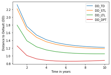
Figure 1 displays the distances to default (DDs) plotted against the number of years until debt maturity (T). The figure indicates that as loan maturity time lengthens, DDs decrease. However, DDs generated using the firm's total debt (TD) are higher than DDs generated using CL, LTL, and DPT. According to this result, businesses that think about using current or short-term liabilities are more likely to default. However, as investment duration increases, the firm's stability to default declines; as a result, this study suggests that firms should think about adopting short-term investments for their stability. The image likewise depicts the DDS and PDs as having an inversely proportional connection. The PDs rise when the DDs fall, and vice versa. 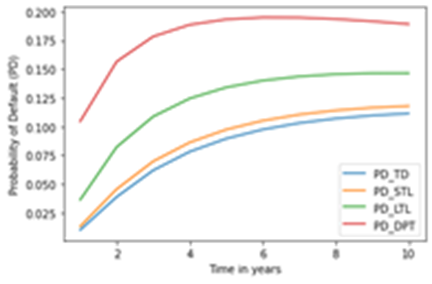This suggests that businesses with larger DDs will experience a decreased likelihood of default. The odds of default are displayed against the dates of the debt maturities in Figure 2 The graph demonstrates that the PDs produced by DPT are more than those produced by TD, CL, and LTL. This result demonstrates that companies utilising DPT in their investment schemes are much more likely to default than companies using TD, CL, or LTL. The image also depicts the exponential rise in default probability before they begin to fall at some point in the future.

Figure 1

                                                                     

Figure 1 Distances to Default vs Time

 

Figure 2

                                                                     

Figure 2 Probability of Default vs Time

 

The impact of altering volatility () on the DDs and PDs is seen in Table 3. The table demonstrates a decline in DDs when volatility rises. This research suggests that because volatility lowers a firm's stability to default, higher volatility firms will default more frequently. The table also demonstrates an increase in PDs as volatility rises, suggesting that businesses with high volatility have a higher chance of defaulting.

Table 3

Table 3 Effect of Volatility on Distance to Default and Probability of Default  from Table 1 (, )
	0.1	0.2	0.3	0.4	0.5	0.6	0.7	0.8	0.9	1.0
	12.8214	6.3357	4.1405	3.0178	2.3243	1.8452	1.4888	1.2089	0.9801	0.7871
	12.2919	6.0709	3.9640	2.8855	2.2184	1.7570	1.4131	1.1427	0.9213	0.7342
	10.1788	5.0144	3.2596	2.3572	1.7958	1.4048	1.1113	0.8786	0.6865	0.5229
	7.4821	3.6661	2.3607	1.6830	1.2564	0.9553	0.7260	0.5415	0.3869	0.2532
	0.0	1.1813e-10	1.7330e-05	1.2729e-03	1.0055e-02	3.2502e-02	6.8274e-02	1.1335e-01	1.6350e-01	2.1560e-01
	0.0	6.3586e-10	3.6859e-05	1.9542e-03	1.3265e-02	3.9461e-02	7.8810e-02	1.2657e-01	1.7844e-01	2.3142e-01
	0.0	2.6599e-07	5.5784e-04	9.2067e-03	3.6266e-02	8.0040e-02	1.3323e-01	1.8981e-01	2.4619e-01	3.0053e-01
	3.6526e-14	1.2315e-04	9.1198e-03	4.6184e-02	1.0448e-01	1.6970e-01	2.3391e-01	2.9407e-01	3.4941e-01	4.0005e-01

 

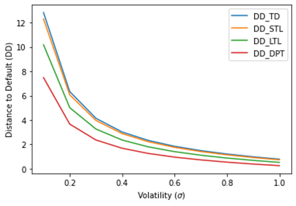
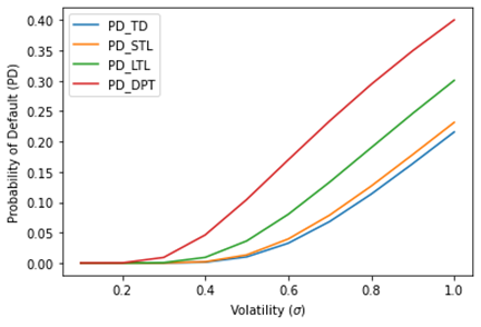
The decline of DDs versus volatilities is depicted in Figure 3 When volatility rises, DDs also fall, and vice versa. The DDs decrease with increasing volatilities. The exponential increase of the PDs versus volatilities is depicted in Figure 4 With rising volatilities, PDs grow exponentially, raising the risk of default.

Figure 3

                                                                    

Figure 3 Distances to Default vs Volatility

 

 

 

 

 

Figure 4

                                                                      

Figure 4 Probability of Default vs Volatility

 

The impact of different interest rates (r) on the DDs and PDs is shown in Figure 4. The table displays the DDs and rates as a  linear relationship. With an increase in interest rates, the DDs rise. This indicates that high interest rates lead to an increase in DDs, making it more likely that the company will eventually default. Lower PDs are seen with higher DDs. The table also demonstrates the decline in PDs in comparison to the rate increase. High interest rates thereby lessen the likelihood of default (PD).

Table 4

Table 4 Effect of Rates on Distance to Default and Probability of Default  from Table 1 (, )
Rate (r)	0.1	0.2	0.3	0.4	0.5	0.6	0.7	0.8	0.9	1.0
	15.7214	7.7857	5.1071	3.7428	2.9043	2.3286	1.9031	1.5714	1.3024	1.0771
	15.1919	7.5209	4.9306	3.6105	2.7984	2.2403	1.8274	1.5052	1.2435	1.0242
	13.0788	6.4644	4.2263	3.0822	2.3758	1.8881	1.5255	1.2411	1.0088	0.8129
	10.3821	5.1161	3.3274	2.4080	1.8364	1.4387	1.1403	0.9040	0.7091	0.5432
	1.7677e-02	1.060e-02	6.1350e-03	3.4223e-03	1.8405e-03	9.5371e-04	4.7610e-04	2.2892e-04	1.060e-04	4.7253e-05
	2.2838e-02	1.3961e-02	8.2341e-03	4.6833e-03	2.5680e-03	1.3571e-03	6.9103e-04	3.3894e-04	1.6011e-04	7.2825e-05
	0.0575	0.0379	0.0241	0.0148	0.0088	0.0050	0.0027	0.0015	0.0007	0.0004
	0.1500	0.1081	0.0754	0.0509	0.0331	0.0209	0.0127	0.0074	0.0042	0.0023

 

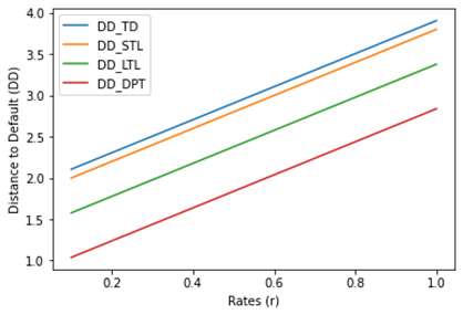
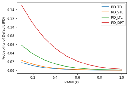
The linear relationship between DDs and rates is depicted in Figure 5. As interest rates rise, the DDs rise as well. Since asset values will be well outside of the default threshold, an increase in DDs implies stability of the firm from default. The inversely proportional link between the PDs and rates is shown in Figure 4 With rising interest rates and vice versa, the PDs decline. This suggests that a high interest rate lowers the risk of a default by the company.

Figure 5

                                                                     

Figure 5 Distances to Default vs Rates

 

Figure 6

                                                                     

Figure 6 Probability of Default vs Rates

 

6. CONCLUSION AND SUGGESTION FOR FUTURE RESEARCH

In this study, the effect of changes in interest rates, volatility, and debt maturity times on the likelihood of default was examined. The study examined the results of the Merton and MKMV strategies for determining the distances to default (DDs) and probability of defaults (PDs). The results show that DDs and PDs produced by the MKMV technique (sDPT) are significant when compared to those produced by the Merton approach in each scenario (sTD, sSTL and sLTL). The DDs appear to be contracting for longer maturities in Figure 1. This shows that as maturities get longer, the company's financial situation gets worse. The development of PDs for longer maturities is seen in Figure 2 This shows that businesses are very vulnerable to defaulting on loans with longer maturities. The decline of DDs versus volatilities is depicted in Figure 3 According to this, asset values converge to the default threshold value as volatilities rise, increasing the chance of default for greater volatilities. The development of the PDs against volatilities is depicted in Figure 4 The likelihood of default rises as volatilities rises. The linear relationship between DDs and rates is depicted in Figure 5. As interest rates rise, the DDs rise as well. Since asset values will be well outside of the default threshold, an increase in DDs implies stability of the firm from default. The inversely proportional link between the PDs and rates is shown in Figure 6. With rising interest rates and vice versa, the PDs decline. This suggests that a high interest rate lowers the risk of a default by the company. Future research will examine the impact of changes in interest rates, volatility, and debt maturity dates on credit ratings and credit quality.

 

CONFLICT OF INTERESTS

None. 

 

ACKNOWLEDGMENTS

None.

 

REFERENCES

Black, F., and Scholes, M. (1973). The Pricing of Options and Corporate Liabilities. Journal of Political Economy, 81(3), 637–654. https://doi.org/10.1086/260062

Chen, X., Wang, X., and Wu, D. D. (2010). Credit Risk Measurement and Early Warning of Smes: An Empirical Study of Listed Smes in China. Decision Support Systems, 49(3), 301–310. https://doi.org/10.1016/j.dss.2010.03.005

Câmara, A., Popova, I., and Simkins, B. (2012). A Comparative Study of The Probability of Default For Global Financial Firms. Journal of Banking and Finance, 36(3), 717–732. https://doi.org/10.1016/j.jbankfin.2011.02.019

Joseph, D. (2021). Estimating Credit Default Probabilities Using Stochastic Optimisation. Data Science In Finance and Economics, 1(3), 253–271.

Joseph, D. (2021). Predicting Credit Default Probabilities Using Bayesian Statistics and Monte Carlo Simulations.

Jumbe, G., and Gor, R. (2022). Estimation of Default Risk by Structural Models : Theory and Literature.

Majumder, D. (2006). Inefficient Markets and Credit Risk Modeling: Why Merton’s Model Failed. Journal of Policy Modeling, 28(3), 307–318. https://doi.org/10.1016/j.jpolmod.2005.10.006

Merton, R. C. (1974). On the Pricing of Corporate Debt: The Risk Structure of Interest Rates. Journal of Finance, 29(2), 449–470. https://doi.org/10.1111/j.1540-6261.1974.tb03058.x

Merton, R. C. (1976). Option Pricing When Underlying Stock Returns Are Discontinuous. Journal of Financial Economics, 3(1–2), 125–144. https://doi.org/10.1016/0304-405X(76)90022-2

Mišanková, M., Kočišová, K., and Adamko, P. (2014). Creditmetrics and Its Use For the Calculation of Credit Risk. In 2nd International Conference on Economics and Social Science (ICESS 2014), Information Engineering Research Institute, Advances In Education Research, 61.

Peresetsky, A. A., Karminsky, A. A., and Golovan, S. V. (2011). Probability of Default Models of Russian Banks. Economic Change and Restructuring, 44(4), 297–334. https://doi.org/10.1007/s10644-011-9103-2

Sariev, E., and Germano, G. (2020). Bayesian Regularized Artificial Neural Networks For the Estimation of the Probability of Default. Quantitative Finance, 20(2), 311–328. https://doi.org/10.1080/14697688.2019.1633014

Tudela, M., and Young, G. (2005). A Merton-Model Approach To Assessing the Default Risk of UK Public Companies. International Journal of Theoretical And Applied Finance, 08(6), 737–761. https://doi.org/10.1142/S0219024905003256

Valášková, K., and Klieštik, T. (2014). Assessing Credit Risk by Merton Model. In Proceedings of The ICMEBIS 2014 International Conference on Management, Education, Business, and Information Science. Edugait Press. Canada, 27–30.

Voloshyn, I. (2015). Usage of Moody’s KMV Model To Estimate A Credit Limit For A Firm. Available at SSRN 2553706. SSRN Electronic Journal. https://doi.org/10.2139/ssrn.2553706

Zieliński, T. (2013). Merton’s and KMV Models In Credit Risk Management. Studia Ekonomiczne, 127, 123–135.