Calibration of Quantum harmonic oscillator as a stock return distribution model on the Index of NSEI

 

Atman Bhatt ¹ , Ravi Gor ²

 

¹ Research Scholar, Department of Applied Mathematical Science, Actuarial Science and Analytics, Gujarat University, Ahmedabad, India

² Department of Applied Mathematical Science, Actuarial Science and Analytics, Gujarat University, Ahmedabad, India

 

1. INTRODUCTION

Standard stochastic process models do not match the results of empirical evidence. Instead of standard financial models, this paper calibrates stock distribution using quantum harmonic oscillator model because the stochastic dynamics of stock return can be studied using quantum models, which can also be used to define its statistical characteristics. The inclusion of market conditions gives quantum models an edge over conventional stochastic models. Quantum harmonic oscillator is the quantum counterpart of the classical harmonic oscillator. It is one of the most crucial model systems in quantum mechanics because it may frequently be represented as a harmonic potential at a stable equilibrium point. It is also one of the few quantum-mechanical systems that has a precise, analytical solution and the market force that pulls a stock return from short-term oscillations to the long-term equilibrium can also be captured by the quantum harmonic oscillator with ease.

 

2. Literature Review

Grabert et al. (1988) proposed generalisation of the Feynman-Vernon impact functional by applying functional integral methods to the quantum mechanical dynamics of a particle connected to a heat bath. The time evolution of equilibrium correlation functions and non-factorizing beginning states is described by the extended theory. Exact solvable models shed light on the theory.

Ye and Huang (2008) suggested a non-classical oscillator model based on Quantum Mechanics. He studied fluctuations of stock markets. Since the same stock has a price range rather than a set price at different times, it is expected that the value might be a packet of trends that determines the possibilities of each price.

Meng et al. (2015) use a quantum spatial-periodic harmonic model to examine the stock market behaviours of equities in daily price-limited stock markets. The effectiveness of price limits is reconsidered, and quantum model is employed to study several observable characteristics of China's price-limited stock markets.

Meng et al. (2016) built an econophysical ‘outline for the stock market using the physical ideas and mathematical constructions of quantum mechanics. Using this framework, he analogously mapped a large number of individual stocks into a reservoir made up of numerous quantum harmonic oscillators, and their stock index into a typical quantum open system, or quantum Brownian particle.

Ahn et al. (2018) developed a quantum harmonic oscillator as a model for the market force that pulls a stock return from short-run oscillations to the long-run equilibrium. Additionally, using analogies, they established an economic justification for physics notions like the eigenstate, eigenenergy, and angular frequency, which clarifies the connection between the literature on finance and econophysics.

Jeknić-Dugić et al. (2018) pursued the quantum-mechanical challenge to the efficient market hypothesis for the stock market by employing the quantum Brownian motion model. He also introduced the external harmonic field for the Brownian particle and use the quantum Caldeira-Leggett master equation as a potential phenomenological model for the stock market price fluctuations.

Lee et al. (2020) examined the weak-form efficient market hypothesis of the crude palm oil market by adopting the quantum harmonic oscillator. This method permits Lee to analyse market efficiency by approximating one constraint: the probability of finding the market in a ground state where conclusion established that the crude palm oil market is more efficient than the West Texas Intermediate crude oil market.

Orrell (2020) addressed issues regarding intrinsically uncertain demand by consuming a quantum context to model supply and demand as, not a cross, but a probabilistic wave, with an allied entropic force. The approach is used to derive from first principles a technique for modelling asset price changes using a quantum harmonic oscillator, that has been previously used and empirically tested in quantum finance. The method is established for a simple system and claims in other areas of economics are discussed.

Bhatt and Gor (2022) showcased an interesting structure of Risk Neutral system. They also examine single step and multistep quantum binomial option pricing model. This approach elaborates circuit proposed by A. Meyer. Bhatt and Gor (2022) review applications of quantum harmonic oscillator model in financial mathematics and also discussed about different applications of quantum harmonic oscillator and its characteristics.

 

3. Data Collection

To calibrate quantum harmonic oscillator model; daily, weekly, and monthly dataset is implemented from Nifty Index of India, spanning 1^st January 2021 to 1^st January 2022 from yahoo-finance.

 

4. Methodology

Firstly, stock returns for different holding periods are calculated and also some insights about the data were found with the help of statistical software Jamovi.

 

4.1. Summary statistics of stock returns for different holding periods

 

 

=1,5 and 20 holding periods Table 1

Table 1

Table 1 Data Exploration
Summary Statistics of Stock Returns for Different Holding Periods
Holding Period	1	5	20
Number of Observation	248	53	12
Mean	0.101	0.0956	0.110
Median	0.134	0.0669	0.0545
Standard deviation	1.09	0.452	0.190
Variance	1.18	0.205	0.0359
Minimum	-4.21	-1.19	-0.217
Maximum	5.08	1.65	0.456
Skewness	-0.248	0.404	0.437
Std. error skewness	0.155	0.327	0.637
Kurtosis	2.76	2.57	-0.0349
Std. error kurtosis	0.308	0.644	1.23

4.2. Parameters of Quantum Harmonic Oscillator

Wiener process is considered to introduce the probability distribution function which is obtained by the Fokker-Planck Equation. Diffusion coefficient is considered as half of the value of the variance which is used to solve the FP Equation and the mass of the Schrodinger equation.

This whole process is supposed to be a time-independent process. Stationary density function is found with the help of time-independent potential and normalization constant.

This all observations are done with fixing value of speed for mean reversion which is equal to. After that angular frequency is calculated which gives insights about from which point the price for a security begins to increase. Five different states are defined considering different five eigenvalues which are derived by the obtained solution of the FP equation.

Probabilities of respective eigenvalues are obtained with the normalization factor which shows the probability of a stock return residing theeigenstate.

Probability density function of the calibrated model is treated as a product of the eigenvalues and its density function. Same process is followed for different holding periods (i.e., 1, 5 and 20 Days).

Calculated values for the above-mentioned parameters of quantum harmonic oscillator and its probability density function are given below. Table 2, Table 3, Table 4.

Table 2

Table 2 Daily Observations
Holding Period	1
Mass
Number of observations	248
angular frequency
-Factor	0.0054
Diffusion Coefficient	0.59
Harmonic Potential	0.00009077
Planck Constant
State	0	1	2	3	4
Energy	0.005431	0.016294	0.027157	0.03802	0.048883
Hermite Polynomial	1	0.06106	-1.98509	-0.7309	11.82126
Amplitude	10.42247	18.05224	23.30534	27.57525	31.2674
Eigen Function	0.232652	0.010045	-0.11546	-0.02454	0.140348
Eigen Value	0.561134	0.67982	0.434081	0.207416	0.082253
Probability	0.310144	0.455218	0.185598	0.042375	0.006664
Density Function	0.999906	0.061054	-1.9849	-0.73083	11.82015
Probability Density Function	0.561081	0.041506	-0.86161	-0.15159	0.972242

 

Table 3

Table 3 Weekly Observations
Holding Period	5
Mass
Number of observations	53
angular frequency
-Factor	0.0023
Diffusion Coefficient	0.1025
Harmonic Potential	0.002263846
Planck Constant
State	0	1	2	3	4
Energy	0.0022638	0.006792	0.011319	0.01585	0.02037
Hermite Polynomial	1	0.028415	-1.999192	-1.147177	11.99031
Amplitude	6.728813	11.65465	15.046083	17.80277	20.18644
Eigen Function	0.289534	0.00582	-0.204649	-0.047941	0.17716
Eigen Value	0.55784	0.66792	0.421490	0.19904	0.07801
Probability	0.317324	0.45492	0.181157	0.040399	0.006205
Density Function	0.999798	0.02841	-1.998789	-1.146946	11.9879
Probability Density Function	0.557727	0.01898	-0.842466	-0.228289	0.93515

 

Table 4

Table 4 Monthly Observations
Holding Period	12
Mass
Number of observations	12
angular frequency
-Factor	0.0009474
Diffusion Coefficient	0.01795
Harmonic Potential	0.000011463
Planck Constant
State	0	1	2	3	4
Energy	0.00095	0.00284	0.00474	0.00663	0.00853
Hermite Polynomial	1.00000	0.05054	-1.99745	-0.60637	11.87739
Amplitude	4.35285	7.53936	9.73327	11.51656	13.05855
Eigen Function	0.35990	0.01286	-0.25417	-0.03150	0.21814
Eigen Value	0.55781	0.66782	0.42138	0.17203	0.06082
Probability	0.32144	0.46073	0.18344	0.03057	0.00382
Density Function	0.99936	0.05051	-1.99617	-0.60598	11.86981
Probability Density Function	0.55746	0.03373	-0.84116	-0.10425	0.72194

 

4.3. Using Goodness of fit test for Parameter estimation of Quantum Harmonic Oscillator

The Cramer–von Mises criterion is a criterion used for adjudicating the goodness of fit of a cumulative distribution function. For goodness of fit test, mean and standard deviation are used to find the value of t-test where mean is summation of products of eigenvalues and its probabilities respectively.

P-values for the given holding periods are zeroes which indicates the curve fitting for the historical data taken. Table 5

Table 5

Table 5 Cramer Von Mises Test
Number of observations	248	53	12
Holding Period	1	5	20
Mean	0.101	0.0956	0.110
Standard deviation	1.09	0.452	0.190
Quantum Harmonic Oscillator
Mean	0.114680	0.113148	0.113955
Variance	0.016717	0.016385	0.016973
Standard deviation	0.129294	0.128003	0.130280
PDF	0.561635	0.441095	0.367726
Cramer Von Mises Goodness of fit Test
T	12.7637	2.11028	4.93087
Standard deviation	0.129294	0.128003	0.130280
z-stat	85.6215	14.1562	33.0773

 

To compare the fitting results of the Cramer Von Mises goodness of fit statistic, following ways are calculated: First, to determine the 5th, 10th, and up to 100th percentiles of returns. The actual number  of empirical returns were evaluated, falling between the 5 and the 5 percentiles and evaluated by:

 

 

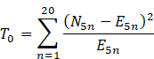
where is mean return falling between the fixed percentiles. Here degree of freedom for the respective model is 14 and in the case of quantum harmonic oscillator all the three p-values of daily, weekly, and monthly data are observed to be greater than 0.05 which is calculated by the found value of z-stat. So, the null hypothesis that the data comes from the distribution of the quantum harmonic oscillator model cannot be rejected.

 

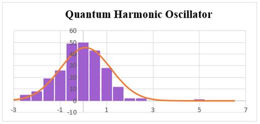
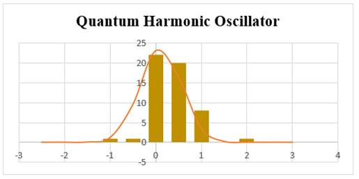
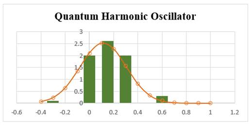
4.4. Graphical representation of Goodness of fit Test

Graphical representations of the goodness of fit test are constructed with MS Excel where annual log-return is used to find respective bins and data. It is distributed normally with the mean and standard deviation derived from quantum harmonic oscillator model.  Figure 1, Figure 2, Figure 3.

Figure 1

                                                                    

Figure 1 Daily Observations

 

Figure 2

                                                                    

Figure 2 Weekly Observations

 

Figure 3

                                                            

Figure 3 Monthly Observations

 

5. Conclusion

The results derived from the quantum harmonic oscillator model indicates a modest but distinct possibility of observing the particle in the traditionally forbidden zone. Quantum harmonic oscillator gives many insights about stock listing of NIFTY50 like diffusion coefficient, Amplitude, Harmonic potential which actually helps to find the Eigen values and its probabilities. Mean value of the quantum harmonic oscillator is nearer to the mean value of the stock return. Prior is the reason for which QHO gives identical values for Cramer-Von Mises Goodness of fit Test and it can be observed from the graphs of different holding periods.

 

CONFLICT OF INTERESTS

None. 

 

ACKNOWLEDGMENTS

None.

 

REFERENCES

Ahn, K., Choi, M., Dai, B., Sohn, S., and Yang, B. (2018). Modeling Stock Return Distributions with a Quantum Harmonic Oscillator. EPL (Europhysics Letters), 120(3), 38003. https://doi.org/10.1209/0295-5075/120/38003.

Bhatt A., and Gor R. (2022). A Review Paper on Quantum Harmonic Oscillator and Its Applications in Finance. IOSR Journal of Economics and Finance (IOSR-JEF), 13 (3), 61-65.

Bhatt A., and Gor R. (2022). Examining Single Step and Multistep Quantum Binomial Option Pricing Model. IOSR Journal of Economics and Finance (IOSR-JEF), 13 (3), 52-60.  

Garrahan, J. (2018). A Comparison of Stock Return Distribution Models.

Grabert, H., Schramm, P., and Ingold, G. L. (1988). Quantum Brownian Motion : The Functional Integral Approach. Physics Reports, 168(3), 115-207. https://doi.org/10.1016/0370-1573(88)90023-3.

Jeknić-Dugić, J., Petrović, I., Arsenijević, M., and Dugić, M. (2018). Quantum Brownian Oscillator for the Stock Market. Arxiv Preprint. https://doi.org/10.48550/arXiv.1901.10544.

Lee, G. H., Joo, K., and Ahn, K. (2020). Market Efficiency of the Crude Palm Oil: Evidence from Quantum Harmonic Oscillator. In Journal of Physics: Conference Series. IOP Publishing. 1593 (1), 012037. https://doi.org/10.1088/1742-6596/1593/1/012037.

Meng, X., Zhang, J. W., Xu, J., and Guo, H. (2015). Quantum Spatial-Periodic Harmonic Model for Daily Price-Limited Stock Markets. Physica A : Statistical Mechanics and its Applications, 438, 154-160. https://doi.org/10.1016/j.physa.2015.06.041.

Meng, X., Zhang, J. W., and Guo, H. (2016). Quantum Brownian Motion Model for the Stock Market. Physica A: Statistical Mechanics and its Applications, 452, 281-288. https://doi.org/10.1016/j.physa.2016.02.026.

Orrell, D. (2020). A Quantum Model of Supply and Demand. Physica A : Statistical Mechanics and its Applications, 539, 122928. https://doi.org/10.1016/j.physa.2019.122928.

Orrell, D. (2021). A Quantum Oscillator Model of Stock Markets. https://doi.org/10.2139/ssrn.3941518.

Ye, C., and Huang, J. P. (2008). Non-Classical Oscillator Model for Persistent Fluctuations in Stock Markets. Physica A : Statistical Mechanics and its Applications, 387(5-6), 1255-1263. https://doi.org/10.1016/j.physa.2007.10.050.