THE EPIDEMIC CONTROL PROCESS, THE CORONA VIRUS, MATHEMATICAL MODELING
Sandy Sánchez Domínguez 1![]()
![]() ,
Adolfo Fernández García 1
,
Adolfo Fernández García 1![]() , Antonio Iván Ruiz Chaveco 2
, Antonio Iván Ruiz Chaveco 2![]()
![]()
1 Faculty of Mathematics and Computation,
U O, Brazil
2 University of the State of Amazonas,
Brazil
|
|
|
ABSTRACT |
|
|
In the present work, a study is made of the development of epidemics, in particular the one referring to the epidemic transmitted by SAR CoV 2; a model is developed through a system of Differential Equations that simulates this process, the system is simplified, if it makes a qualitative study of the trajectories of the system giving conclusions regarding the hole behavior of the trajectories, thus proving control of the epidemic; a critical case is treated and an example is presented that responds to the conditions of the introduced critical case, graphically proving the conclusions demonstrated analytically. |
|||
|
Received 03 December 2022 Accepted 02 January 2023 Published 18 January 2023 Corresponding Author Antonio
Iván Ruiz Chaveco, iruiz2005@yahoo.es DOI 10.29121/IJOEST.v7.i1.2023.418 Funding: This research
received no specific grant from any funding agency in the public, commercial,
or not-for-profit sectors. Copyright: © 2023 The
Author(s). This work is licensed under a Creative Commons
Attribution 4.0 International License. With the
license CC-BY, authors retain the copyright, allowing anyone to download,
reuse, re-print, modify, distribute, and/or copy their contribution. The work
must be properly attributed to its author.
|
|||
|
Keywords: Coronavirus,
Epidemic, Mathematical Model |
|||
1. INTRODUCTION
This work is fundamentally related to the epidemic produced by SAR CoV 2 but is applicable to epidemics transmitted by other diseases with person-to-person contagion, such is the case of sexually transmitted diseases where the fundamental difference is that the concentrations between susceptible and exposed are very minor Soto et al. (2019) and Soto et al. (2020).
Multiple diseases that develop epidemics are known Halloran et al. (1994), Halloran et al. (1994), Hamer et al. (1906) and Hethcote (1994). But for its lethality COVID 19 finds itself in the worst cases for human health Lacort et al. (2020).
The disease that has most affected humanity in recent years has been COVID-19. It is said that the cases of maximum risk are adults of the third age and especially those who suffer from some chronic disease; but practice has shown that there is no one safe from this disease, and it can have a slow evolution or act swiftly.
Due to these great affects produced by COVID-19 in the world, multiple results have been published both from the point of view of biochemical characteristics, of treatment, and from the point of view of modeling to make predictions regarding the future of the pandemic, among others can be indicate the works Ramirez-Torres et al. (2020), Ivorra et al. (2020), Ruiz Aa and Marténig (2020) and Zhao and Chen (2020), which represent models through ordinary differential equations, which give conclusions regarding the future behaviour of the infection process of the population considered.
Today the most worrying situation is given by the coronavirus, a respiratory disease that so many lives have claimed, there are many ideas on how to fight this disease; but the method that most researchers agree on, is given by the method of isolating the infected to prevent possible transmission to other people Montero (2020).
In Chaveco et al. (2018) different problems of real life are treated by means of equations and systems of differential equations, all of them only in the autonomous case; where examples are developed, and other problems and exercises are presented for them to be developed by the reader.
The authors of Chaveco et al. (2016) indicate a set of articles forming a collection of several problems that are modelled in different processes, but in general the qualitative and analytical theory of differential equations is used both in the autonomous and non-autonomous cases, in both books the authors address the problem of epidemic development.
There are multiple works dedicated to the study of the causes and the conditions under which an epidemic may develop, among these we can indicate Hamer (1906).
The first navigators who arrived in the Americas were impressed with the robustness and the healthy aspect of the Indians, who, in fact, fed abundantly on natural products, moved constantly, therefore had no problems of sedentary lifestyle, and did not cultivate habits harmful to health. Tobacco, for example, was used only sporadically and in rituals; the problems later created by the industrialization, commercialization and advertising of cigarettes that did not exist. This picture soon began to change; the Europeans brought with them, in addition to economic interest and firearms, microbes that caused diseases to which the Indians had no immunity.
That way they could get seriously ill, and even die, from a simple flu. Other diseases were even worse, such as smallpox, a disease that no longer exists; it disappeared after a successful worldwide vaccination campaign, conducted by the World Health Organization more than 40 years ago. But at that time the vaccine did not exist and, even if it did, it would not be applied to the Indians Other diseases from the Old World were being introduced: malaria, yellow fever, tuberculosis, bubonic plague. Soon the entire population of the colony was subject to them; black slaves, because of the poor conditions of life and nutrition; whites, because they lacked effective vaccines or treatments.
To this was added another factor: the emergence of cities, which had precarious conditions of hygiene and sanitation. With regard to organized public health, little was done, there was a chief physicist, who, through assistants, supervised medical practice, and the sale of medicines was carried out at apothecaries, which still used leeches, which were used to extract the “excess” of blood or “poisoned” blood.
The problem of epidemic modeling has always been of great interest to researchers such as the cases of Esteva and Vargas (1998), Earn et al. (2000), Greenhalgh and Das (1992), Gripenberg (1983), Halloran et al. (1994), Halloran et al. (1994), Hethcote (1994) and Hethcote (1976). In this work we will apply the generalized logistic model, where the case of the growth and decrease of the infected are applied in the same equation; to model the development of epidemics, a model that allows forecasts of future behaviour.
The objective of this work is to perform a modelling using ordinary differential equations, the infection process using COVID-19 in such a way that it can respond to the current situation in different countries and regions where the problem of multiple waves is presented; as it happened in Cuba and other countries, a possibility that had already been indicated in Ruiz Aa And Marténig (2020), where in addition it was planted how to reverse this situation.
2. MODEL FORMULATION
The process of infection through the coronavirus until effective measures are not taken has an exponential growth, with many infected individuals appearing quickly, leading to the death of many of them if they do not receive adequate treatment. It is known that to study a model that simulates the process it is necessary to see how the infected will vary over time; here the situation will be analyzed when they are in the process of growing or decreasing as a result of the treatment.
The disease that most affected humanity in recent years was COVID-19. It is said that the highest risk cases are elderly adults and especially those who suffer from a chronic disease; but practice has shown that no one is safe from this disease, that it can evolve slowly or act quickly, that anyone can be infected and from that moment on it is not possible to say what the patient's future will be.
The infection process through the coronavirus increases proportionally to the concentration of exposed people and its own concentration, decreasing proportionally to the population of recovered. Susceptible will increase proportionally to their concentration up to a certain value, as they can pass through their immune system directly to recovered ones, and it decreases proportionally to the amount of exposed; the exposed population decreases proportionally to its concentration and decreases proportionally to the concentration of infected, adding proportionally to the susceptible population; the recovered population decreases in proportion to the infected population.
To formulate the model using a system of differentiable equations, the following unknown functions will be introduced:
𝑖1̃ is the total concentration of the infected population at the time 𝑡.
s̃1 is the total concentration of the susceptible population at the time 𝑡.
ẽ1 is the total concentration of the exposed population at the time 𝑡.
r̃1 is the total concentration of the population recovered at the time 𝑡.
In addition, the open set 𝑉𝛼 will be denoted by,
![]()
This set represents the region of admissible values of populations at a given time.
Here the variables will be introduced ![]() ,
,
![]() ,
,
![]() and
and ![]() defined as follows:
defined as follows: ![]() ,
,
![]() ,
,
![]() and
and ![]() ;
so if
;
so if ![]() ,
,
![]() ,
,
![]() and
and ![]() the following conditions
would be satisfied
the following conditions
would be satisfied ![]() ,
,![]() ,
,![]() and
and ![]() which would constitute the
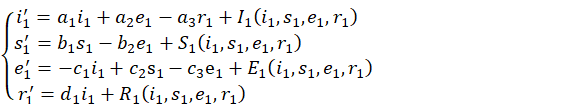
main objective of this epigraph. Considering the above principles, the
mathematical modeling of the coronavirus infection process takes the following form,
which would constitute the
main objective of this epigraph. Considering the above principles, the
mathematical modeling of the coronavirus infection process takes the following form,
Equation 1
With the initial conditions,
![]() ,
,
![]() ,
,
![]() .
.
Where I1, S1, E1 and 𝑅1 will represent disruptions to the infection process, which ultimately could produce significant changes in the numbers of individuals in each of the classifications, such as infected, susceptible, exposed and recovered, as it is assumed that once the pandemic appears, it will not disappear completely. These functions are power series converging in a neighbourhood of the origin of coordinates, which have the following representation,
![]() ,
,
![]()
Likewise, for, 𝑆1, 𝐸1 and 𝑅1.
The parameters that appear in the system correspond to:
𝑎1 is the coefficient of increase in the concentration of the infected due to their own concentration.
𝑎2 is the coefficient of increase in the concentration of those infected as a function of the concentration of those exposed.
𝑎3 is the coefficient of decrease in the concentration of the infected as a function of the concentration of the recovered.
𝑏1 is the coefficient of increase in the concentration of susceptible as a function of their own concentration.
𝑏2 is the coefficient of decrease in the concentration of susceptible as a function of the concentration of those exposed.
𝑐1 is the coefficient of decrease in the concentration of those exposed as a function of their own concentration.
𝑐2 is the growth coefficient of the concentration of the exposed as a function of the concentration of the susceptible.
𝑐3 is the coefficient of decrease in the concentration of those exposed as a function of their own concentration.
𝑑1 is the growth coefficient of the concentration of the recovered as a function of the concentration of the infected.
The characteristic equation corresponding to the matrix of the linear part of the system Equation 1 has the form,
![]() Equation 2
Equation 2
Where,
![]()
![]()
![]()
![]()
Theorem 1: The conditions ![]() ,
,
![]() and 𝑛3
and 𝑛3 ![]() are necessary and sufficient for the trivial
solution of system Equation 1
to be asymptotically stable. The proof of this theorem is a direct consequence
of the Hurwitz conditions, which guarantee the negativity of the real parts of
the roots of the characteristic equation, in correspondence with the method of
the first approximation.
are necessary and sufficient for the trivial
solution of system Equation 1
to be asymptotically stable. The proof of this theorem is a direct consequence
of the Hurwitz conditions, which guarantee the negativity of the real parts of
the roots of the characteristic equation, in correspondence with the method of
the first approximation.
Observation 1: Theorem1 allows us to state that
under the conditions ![]() ,
,
![]()
![]() the infection is controlled, because although
the active cases are not eliminated, there is also no epidemic, since the total
concentrations of the populations in each of the statuses converge to
acceptable values of the corresponding populations. Could it be the case that
the infection is controlled, because although
the active cases are not eliminated, there is also no epidemic, since the total
concentrations of the populations in each of the statuses converge to
acceptable values of the corresponding populations. Could it be the case that ![]() ,
, ![]() and
and ![]() ,
if this occurs, we would have that among the eigenvalues of the matrix of the
linear part of the system there is a negative, a null and a pure imaginary
double, thus constituting a critical case, which could not be solved by
applying the method of first approximation; here it will be necessary to reduce
the system to a simpler form and apply the second Lyapunov method to draw
conclusions regarding the future of the disease.
,
if this occurs, we would have that among the eigenvalues of the matrix of the
linear part of the system there is a negative, a null and a pure imaginary
double, thus constituting a critical case, which could not be solved by
applying the method of first approximation; here it will be necessary to reduce
the system to a simpler form and apply the second Lyapunov method to draw
conclusions regarding the future of the disease.
By means of a non-degenerate transformation X = SY, where ![]() and
and ![]() ,
the system Equation 1
can be transformed into the system,
,
the system Equation 1
can be transformed into the system,
Equation 3
The functions ![]() ,
,
![]() ,
,![]() and
and ![]() admit a converging power
series development in a neighbourhood of the origin of the coordinates,
similarly to what was indicated before, for the functions,
admit a converging power
series development in a neighbourhood of the origin of the coordinates,
similarly to what was indicated before, for the functions, ![]() ,
,
![]() ,
,![]() and
and ![]() ,
so,
,
so,
![]()
Likewise, for the rest.
In this case, because it is a critical case, the Analytical Theory of Differential Equations will be applied to simplify the system.
Theorem 2: The change of variables,
Equation 4
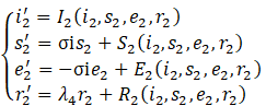
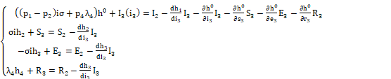
transforms the system Equation 3 into the combined quasi-normal form,
Equation 5
Where ![]()
![]() ,
,![]()
![]() and
and ![]() admit a development similar to
admit a development similar to ![]() ,
,
![]() ,
,![]() and
and ![]() ,
furthermore
,
furthermore ![]() and
and ![]() cancel for
cancel for ![]() .
.
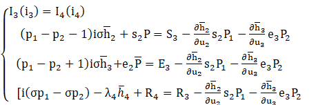
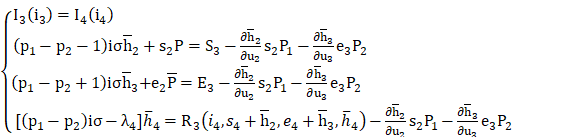
Proof: Deriving the transformation Equation 4 along the trajectories of systems Equation 3 and Equation 5 we obtain the following system of equations,
Equation 6
To determine the series that intervene in the systems and
in the transformation, the coefficients of the powers of grade ![]() in the following two cases: Case I) Doing
in the following two cases: Case I) Doing ![]() in system Equation 6,
that is to say for the vector
in system Equation 6,
that is to say for the vector ![]() the following system is obtained,
the following system is obtained,
Equation 7
The system Equation 7
allows to determine the coefficients of the series, ![]() and
and ![]() where for being the resonant case
where for being the resonant case ![]() ,
and the other series are determined in a unique way. Case II) For the case when
,
and the other series are determined in a unique way. Case II) For the case when
![]() of the system Equation
6
it follows that,
of the system Equation
6
it follows that,
Equation 8
As the series of the system Equation 3
are known expressions, the system Equation 8
allows to calculate the series ![]() ,
,
![]() ,
, ![]() and
and ![]() .
This proves the existence of change of variables.
.
This proves the existence of change of variables.
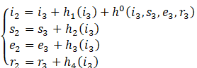
Theorem 3: The transformation of coordinates,
Equation 9
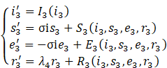
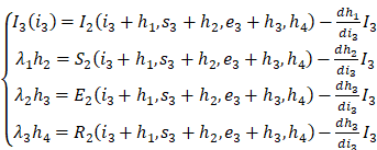
reduces system Equation 5 to the combined quasi-normal form,
Equation 10
Where ![]() and the functions
and the functions ![]() are uniquely determined.
are uniquely determined.
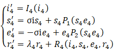
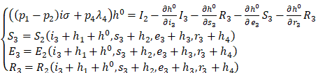
Proof: Deriving the transformation Equation 9 along the trajectories of systems Equation 5 and Equation 10 we obtain the system of equations,
Equation 11
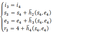
Doing in the system Equation 11 𝑟4 = 0, the system is obtained,
Equation 12
The system Equation 12
allows calculating the series ![]() ,
,
![]() and
and ![]() with what
with what ![]() and
and ![]() are nonzero in the resonant case, that is,
their exponents satisfy the resonance equations
are nonzero in the resonant case, that is,
their exponents satisfy the resonance equations ![]() and
and ![]() ,
this guarantees the form previously indicated for these series; meantime,
,
this guarantees the form previously indicated for these series; meantime, ![]() ,
,
![]() and
and ![]() because they are not resonant, they are
uniquely determined. When
because they are not resonant, they are
uniquely determined. When ![]() ,
from the system Equation
11
the equation is deduced
,
from the system Equation
11
the equation is deduced ![]() ,
this completes the proof of the theorem, since the unknown series are thus
calculated.
,
this completes the proof of the theorem, since the unknown series are thus
calculated.
In system Equation 11
the functions ![]() and
and ![]() admit the following power series development:
admit the following power series development:
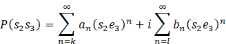
and
![]()
Theorem 4:
If ![]() ,
,
![]() e
e
![]() ,
,
![]() ,
𝑠
odd and
,
𝑠
odd and ![]() , then the trajectories of system Equation 10
are asymptotically stable, otherwise they are unstable.
, then the trajectories of system Equation 10
are asymptotically stable, otherwise they are unstable.
Proof: Consider the positive definite Lyapunov function,
![]()
The function 𝑉(𝑢1, 𝑢2, 𝑢3) is such that its derivative along the trajectories of the system (10) has the following expression,
![]()
This function is negative definite because in 𝑅 the powers are of degrees higher than those indicated in the initial part of the expression for the derivative of 𝑉, this allows us to state that the equilibrium position is asymptotically stable.
Note2: If 𝑛𝑖 > 0, 𝑖 = 1,2,3, 𝑛1𝑛2 = 𝑛3 and 𝑛4 = 0, 𝛼 < 0, 𝑠 odd and 𝑎𝑘 < 0 then, the total concentrations of populations in each of the statuses converge to the admissible values; thus, there will be no danger of the development of an epidemic, as the disease still exists, it will remain under control.
Example: Let the following system simulate the process of coronavirus infection in a given population.
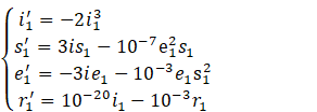
With the initial conditions,
![]() ,
,
![]()
![]()
Figure1
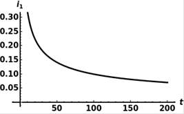
|
Figure 1 Graph of 𝒊𝟏 with respect 𝒕. |
Figure 2
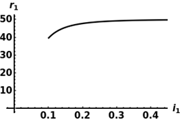
|
Figure 2 Graph of 𝒓𝟏 with respect 𝒊𝟏 |
Note 3: From the graph of Figure 1, from the example, it can be seen that the concentration of the infected population decreases over time, this result corresponds to reality, as these values will decrease over time due to treatment, or personal immunity, because here the conditions of theorem4 are satisfied.
Note 4: From the graph in Figure 2, from the example, it can be seen that the concentration of the recovered population grows to a maximum value as a result of the treatment or the immunity of certain members of the population, this is in line with reality, as the conditions are met. of stability. VI.
3. CONCLUSION
1)
Due to the danger to
human life, it is of paramount importance to study the characteristics of the
coronavirus, the forms of transition and the methods of combating the disease,
which would allow a more effective treatment for patients; this is more evident
nowadays with the appearance of multiple waves, which represents a renewal of
the disease.
2)
Historically, there
have been diseases that, due to their propagation, have become epidemics, but
never with the danger of the coronavirus; and worse with the appearance of new
strains linked to multiple waves.
3)
If the conditions ![]() ,
,
![]() and
and ![]() , are
satisfied then the total concentrations of the populations corresponding to
infected, susceptible, recovered and exposed converge to the ideal
concentrations.
, are
satisfied then the total concentrations of the populations corresponding to
infected, susceptible, recovered and exposed converge to the ideal
concentrations.
4)
If ![]() ,
, ![]() and
and ![]() if there is a critical case for which it is necessary to use the
qualitative theory of differential equations to reach conclusions regarding the
studied process.
if there is a critical case for which it is necessary to use the
qualitative theory of differential equations to reach conclusions regarding the
studied process.
5)
Theorems 3 and 4 give
the technique to be followed to simplify the system corresponding to the model
that simulates the infection process by means of the coronavirus, in the case
where there is a critical case indicated above.
6) If ![]() ,
,
![]() ,
,
![]() ,
,
![]() ,
,
![]() odd and
odd and
![]() ,
then in the critical case considered, the total
concentrations of the infected, exposed, recovered and susceptible population
converge to the admissible concentrations and in this way the infection process
would be controlled.
,
then in the critical case considered, the total
concentrations of the infected, exposed, recovered and susceptible population
converge to the admissible concentrations and in this way the infection process
would be controlled.
7)
Graphs 1 and 2 show in
practice that under the conditions of theorem4 the total concentrations in each
of the statuses converge to ideal values, so given the disease, once a set of
data has been determined, it is necessary to concentrate the resources of
science to achieve that these conditions are met and thus prevent the
development of the epidemic.
CONFLICT OF INTERESTS
None.
ACKNOWLEDGMENTS
None.
REFERENCES
Alraddadi, B. M., Watson, J. T., Almarashi, A., Abedi, G. R., Turkistani, A., Sadran, M., Housa, A., Almazroa, M. A., Alraihan, N., Banjar, A., Albalawi, E., Alhindi, H., Choudhry, A. J., Meiman, J. G., Paczkowski, M., Curns, A., Mounts, A., Feikin, D. R., Marano, N., Madani, T. A. (2016). Risk Factors For Primary Middle East Respiratory Syndrome Coronavirus Illness In Humans, Saudi Arabia, 2014. Emerging Infectious Diseases, 22(1), 49-55. https://doi.org/10.3201/eid2201.151340.
Chaveco, A. I. R. and Others. (2016). Applications of Differential Equations In Mathematical Modeling. V.Um. CRV, 196.
Chaveco, A. I. R. and Others. (2018). Modeling of Various Processes. [Curitiba : Appris], 1, 320.
Earn, D. J. D., Rohani, P., Bolker, B. M., and Grenfell, B. T. (2000). A Simple Model For Complex Dynamical Transitions In Epidemics. Science, 287(5453), 667-670.
Esteva, L., and Vargas, C. (1998). Analysis of A Dengue Disease Transmission Model. Mathematical Biosciences, 150(2), 131-151. https://doi.org/10.1016/s0025-5564(98)10003-2.
Greenhalgh, D., and Das, R. (1992). Some Threshold and Stability Results for Epidemic Models With A Density Dependent Death Rate, Theoret. Population Biol., 42, 130-151.
Gripenberg, G. (1983). On A Nonlinear Integral Equation Modelling An Epidemic In An Age-Structured Population. Journal Für Die Reine Und Angewandte Mathematik, 341, 147-158. https://doi.org/10.1515/crll.1983.341.54.
Halloran, M. E., Cochi, S. L., Lieu, T. A., Wharton, M., and Fehrs, L. (1994). Theoretical Epidemiologic and Morbidity Effects of Routine Varicella Immunization of Preschool Children In The United States. American Journal of Epidemiology, 140(2), 81-104. https://doi.org/10.1093/oxfordjournals.aje.a117238.
Halloran, M. E., Cochi, S. L., Lieu, T. A., Wharton, M., and Fehrs, L. (1994). Theoretical Epidemiologic and Morbidity Effects of Routine Varicella Immunization of Preschool Children in The United States. American Journal of Epidemiology, 140(2), 81-104. https://doi.org/10.1093/oxfordjournals.aje.a117238.
Halloran, M. E., Watelet, L., and Struchiner, C. J. (1994). Epidemiologic Effects of Vaccines With Complex Direct Effects In An Age-Structured Population. Mathematical Biosciences. WATELET, 121(2), 193-225. https://doi.org/10.1016/0025-5564(94)90070-1.
Hamer, W. H. (1906). Epidemic Disease In England. Lancet, 1, 733-739. https://doi.org/10.1016/S0140-6736(01)80187-2
Hamer, W. H. (1906). Epidemic Disease In England: The Evidence of Variability and of Persistency of Type. Bedford Press.
Hethcote, H. W. (1976). Qualitative Analyses of
Communicable Disease Models. Mathematical Biosciences, 28(3-4), 335-356. https://doi.org/10.1016/0025-5564(76)90132-2.
Hethcote, H. W. (1994). A Thousand and One Epidemic
Models. Frontiers in Mathematical Biology. Springer, 504-515. https://doi.org/10.1007/978-3-642-50124-1_29.
Ivorra, B., Ferrández, M. R., Vela-Pérez, M., and Ramos, A. M.
(2020). Mathematical Modeling of The Spread of The Coronavirus Disease
2019 (Covid-19) Tak Ing Into Account The Undetected Infections. The Case of
China. Communications In Nonlinear Science and Numerical Simulation, 88. https://doi.org/10.1016/j.cnsns.2020.105303.
Lacort, M., Sánchez, S., and Ruiz, A. I. (2020). Coronavirus, A Challenge For Sciences, Mathematical Modeling. IOSR Journal of Mathematics, 16, 28-34.
Montero, C. L. A. (2020). "Covid 19 with Science in China".
Ramirez-Torres, E. E., Selva Castañeda, A. R., Rodríguez-Aldana, Y.,
Sánchez Domínguez, S., Valdés García, L. E., Palú-Orozco, A., Oliveros-Domínguez,
E. R., Zamora-Matamoros, L., Labrada-Claro, R., Cobas-Batista, M., Sedal-Yanes,
D., Soler-Nariño, O., Valdés-Sosa, P. A., Montijano, J. I., And Bergues
Cabrales, L. E. (2020). Mathematical Modeling and Forecasting of COVID-19:
Experience In Santiago De Cuba Province. Revista Mexicana De Física, 67,
123-136. https://doi.org/10.31349/RevMexFis.67.123.
Ruiz Aa, L. L. Mc., And Marténig, F. (2020). Rb, Sousa Vf, Andrade Fd, Lima Pe, Iglesiana, Lacortmh, Sánchez Sa, Ruiz A Ib. "Coronavirus, A Challenge For Sciences, Mathematicalmodeling". IOSR Journal of Mathematics, 16(3) Ser. I, 28-34.
Soto, E. Et Al. (2020). Model of Sexually Communicable Diseases With Homosexual Presence. IOSR Journal of Mathematics, 16, 01-06. Model of Sexually Communicable Diseases With Homosexual Presence.
Soto, E., Fernandes, N., Sánchez, S., Leão, L., Ribeiro, Z., Ferreira,
R., and Ruiz, I. (2019). Models of Sexually Transmitted Diseases. European
Journal of Engineering Research and Science, 4(10), 4-8. https://doi.org/10.24018/ejeng.2019.4.10.1543.
Zhao, S., and Chen, H. (2020). Modeling the epidemic dynamics
and control of Covid-19 outbreak in china. Quantitative Biology, 8(1), 11-19. https://doi.org/10.1007/s40484-020-0199-0.
 This work is licensed under a: Creative Commons Attribution 4.0 International License
© Granthaalayah 2014-2023. All Rights Reserved.