Back-testing approaches for Validating VaR models

 

Kirit Vaniya ¹ , Ravi Gor ²

 

¹ Research scholar, Department of Mathematics, Gujarat University, India

² Department of Mathematics, Gujarat University, India

 

1. INTRODUCTION

Risk management is an important segment of an investment strategy. For managing risk, we have plenty of methods. It is also equally important to check the relevancy of an appropriate method. As value at risk (VaR) is mostly used market risk measures. we have various approaches to calculate VaR. To check the mobility of VaR method, back-testing is required. In back-testing original historical return data is compared with predicted VaR data values over the same historical period.

In this article, we will review the methodologies for Back-testing of VaR. VaR is risk indicator that quantifies the extent and probability of possible potential losses as single value on given investment with given probability, on given time horizon for a portfolio. VaR is particularly useful in portfolio optimization, especially optimizing risk. Mostly for VaR we have used confidence level 95% & 99% and considered one day VaR.

There are mainly three methods to estimate value at risk Abad et al. (2014):

1)     Parametric Method: Parametric methods involves statistical factors, such as volatility, distribution etc. it involves different Density functions, and Higher-order conditional time-varying moments. Variance-Covariance is firstly developed parametric method.

2)     Semi-Parametric Method: Semi-parametric methods involve combination of parametric and non-parametric approach. Volatility-weight historical simulation, Filtered Historical Simulation, CAViaR model, Extreme Value Theory, and Monte Carlo Simulation are some of the methods.

We have introduced one more method that combines historical simulation method with fitting of a cubic polynomial to the sorted return data Vaniya and Gor, (2020), Vaniya and Gor (2021). VaR value is predicted by the value of polynomial at corresponding quantile (percentile) value.

3)     Non-Parametric Method: This kind of approaches involves historical parameters, the non-parametric methods involve, Historical Simulation, and non-parametric density estimation methods.

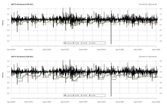
In this paper basic four methods namely Variance Co-variance method, Historical simulation method, Monte-Carlo simulation, and cubic polynomial regression method Vaniya and Gor (2020), Vaniya and Gor (2021) are applied on nifty 50 index for calculating one day VaR. Predicted VaR with original return is given in the image below. We have used both 95% and 99% confidence intervals for one day VaR calculation.

Figure 1

                                                                     

Figure 1 In section 2 of this paper, we have discussed a brief literature on back-testing methods. In the following section 3 we have discussed the back testing method such as Total number of exceptions by binary back-testing function, Basels’ Traffic Light Zone Test, Kupiec POF-test, Kupiec TUFF-test and Haas’ Mixed-Kupiec test. The paper end with conclusion and bibliography.

 

 

 

2. LITERATURE

Validating a VaR model is equally important as predicting VaR estimates. Especially on Indian stock market Yawalkar and Rao (2004) back-tested different VaR methods with different back testing approaches.  There are various approaches for back testing, but they all look at rate that how often an actual return exceeded the one-day VaR. The term “exception” is used for a day where the return is below the predicted VaR estimate. For a confidence level of 95% or 99%, the one-day VaR should be exceeded approximately on 5% or 1% of all days. When there are significantly more (or less) exceptions observed, it can be concluded that model might not be suitable to estimate risk. A good overview on backtesting is provided by Nieppola Nieppola (2009). In general, back-tests are divided into two categories: unconditional coverage tests and conditional coverage Jorion (2007). Kupiec developed the point of failure test (POF-Test) in 1995, which tests the frequency of exceptions, also known as failure rate Kupiec et al. (1995). To take the independence of exceptions into account, Kupiec has also developed a second test, called TUFF-test (time until first failure). Haas Haas (2001) proposed a backtest that considers the time between successive exceptions. He takes advantage of the TUFF test to measure the time in-between exceptions and combines it with the POF test to check if the overall rate of failure is accurate.

Back-testing is a statistical procedure where actual profits and loss are systematically compared to corresponding VaR estimates. For example, if the confidence level used for calculating daily VaR is 99%, we expect an exception to occur once in every 100 days on average. In the back testing process, we could statistically examine whether the frequency of exceptions over some specified time interval is in line with the selected confidence level.

 

3. BACK-TESTING METHODS

There are different methods for back testing, in this paper we discussed four such methods. We have back tested VaR obtained by Variance Co-variance method, Historical simulation method, Monte-Carlo simulation, and cubic polynomial regression method. We have used Total exceptions method by binary function over entire population. We have also used Basel Traffic Light Zone Test, Kupiec POF-test, Kupiec TUFF-test to validate VaR model. We have also discussed about Haas’ Mixed-Kupiec test method.

 

3.1. TOTAL NUMBER OF EXCEPTIONS

The most basic method is of calculating total exceptions or exceptions probability generated for the test period. To calculate total exceptions, we set a binary function that compare the original return with predicted VaR as follows.

Binary function value of any day is defined as

 

 

In this way, we get binary sequence of ones and zeros for the days of test period. Where one denotes the exception. By calculating total number of one in sequence we have total exceptions over test period. We can also get the probability of exception by calculating mean of these sequence (1,1,1,0,0, 1,…) that is required failure rate. i.e. for sequence (1,1,1,0,0, 1,…) where 1 indicates failure and 0 indicate non-failure day

 

 

For NIFTY 50 index in our sample, we have calculated number of failures and failure rate for 95% VaR and 99% VaR.

We have calculated VaR for NIFTY 50 index from all four method and beck tested with failure rate method. Results are given in Table 1.

Table 1

Table 1 Number of Exceptions for NIFTY 50 Index (out of 2834 days data)
Confidence interval	Historical simulation	Analytical method	Monte-Carlo simulation	Cubic polynomial Regression
Failures at 95%	175	147	147	107
Prob.	0.062	0.052	0.052	0.038
Failures at 99%	50	67	63	61
Prob.	0.018	0.024	0.022	0.022

 

3.2. Basel Traffic Light Zone Test (BASEL II coverage test)

It is with the statistical limitations of backtesting in mind that the Basel Committee introduced a framework for backtesting results that encompasses a range of possible BCBS (1996) responses, depending on the strength of the signal generated from the backtest. These responses are classified into three zones, distinguished by colours into a hierarchy of responses. The green zone corresponds to backtesting results that do not themselves suggest a problem with the quality or accuracy of a bank’s model. The yellow zone encompasses results that do raise questions in this regard, but where such a conclusion is not definitive. The red zone indicates a backtesting result that almost certainly indicates a problem with a bank’s risk model.

We have calculated VaR for NIFTY 50 index from all four method and beck tested with Besels’ traffic light zone method. Results are as in Table 3. Corresponding choice of color zone is in Table 2.

Table 2

Table 2 Basel Traffic Light Zone (number of failures for 2834 days)
Confidence int.	Red Zone	Yellow Zone	Green Zone
At 99% confidence	more than 56	Up to 56	Up to 28
at 95% confidence	more than 284	Up to 284	Up to 142

 

Table 3

Table 3 Zone for Number of Exceptions Fnifty 50 Index (out of 2834 days data)
Confidence interval	Historical simulation	Analytical method	Monte-Carlo simulation
95%	Yellow	Yellow	Yellow
99%	Yellow	Red	Red

 

3.3. KUPIEC'S TESTS

Kupiec (1995) has developed two type of back testing methods. A point of failure test (POF-Test) which is unconditional test, that tests the frequency of exceptions. From these exceptions we get failure rate.  For conditional test Kupiec developed TUFF-test (time until first failure) to take the independence of exceptions into account.

These tests give negative results for the exceptions that are too high or too low. It is indicated that these tests must be used with care, taking note of such too high and too low failures cases. In case of too low exceptions, we can say that model is overestimating the risk. And in case of too low exceptions, risk is underestimated. We can accept low exceptions, but too low exceptions are not welcome for accepting the model. These test works better than the Basel traffic light zone test as they check the proportion, occurrence, and the frequency of exceptions. Clear idea for accepting or rejecting the VaR model can be observed when we look at the number of VaR failures, with the Kupiec backtest results. This will clear that whether the given VaR model is underestimating or overestimating risk. All Kupiecs’ test are based on likelihood ratio (LR) test with the ideal LR statistic zero. LR for model gets high when there are cases of too less or too many exceptions either. If this statistic exceeds the critical Chi squared value obtained at the given significance level, we accept the alternate hypothesis in place of the null hypothesis.

For all the three tests the Null hypothesis is as follows

 

 

Here p = significance level = 0.01 or 0.05 corresponding to confidence level of 99% or 95% respectively.

 

3.3.1.  KUPIEC'S POF TEST(UNCONDITIONAL)

It tests expectations frequency, also called a failure rate. The failure rate should match with the corresponding VaR confidence level chosen. If there are more or fewer failure than expected, then VaR model underestimate or overestimate risk respectively.

The failure rate is defined as  where,  is number of failures, and  is total number of observations. For a selected VaR confidence level of 95% or 99%, the failure rate should converge to 5% or 1% respectively (which is p =1- confidence level) when the total number of observations is increased Jorion (2007). The total amount of VaR violations follows a binomial probability distribution:

 

 

           This can be approximated by normal distribution:

 

 

 

 

Based on this distribution, one can test the null hypothesis that

 

 

If we can show that x/T is significantly different from p, we should reject the VaR model. The POF test is a likelihood radio test, were,

 

 

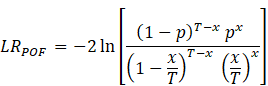
, Likelihood ratio should be chi-squared distributed, using one degree of freedom. The VaR model will be rejected if the likelihood radio statistic exceeds the critical value of the chi-squared distribution.

This test has two problems:

1)     the test performance is weaker in case of smaller samples. And

2)     it cannot observe the exceptions in Cluster as already described above.

Hence other backtests have been developed.

VaR for NIFTY 50 index from all four method is calculated and beck tested with Kupiec-POF method. Results of  for Null Hypothesis  are as in table 4.

Table 4

Table 4 results for Null Hypothesis (out of 2834 days data)
Confidence interval	Historical simulation	Analytical method	Monte-Carlo simulation
95%	Accept	Accept	Accept
99%	Reject	Reject	Reject

 

3.3.2.  KUPIEC'S TUFF TEST (CONDITIONAL)

Kupiec has also developed a second test which takes time of first exception into consideration. This second test is called Kupiec’s TUFF-test (time until first failure) Kupiec et al. (1995). The Likelihood-ratio for the TUFF test is:

 

 

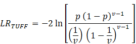
where p is equal to confidence level), and  is the time until the first exception. As in this test only first failure is considered, it do not discover the clustering of failures in the data in between.

To resolve this Haas Haas (2001) has developed another method as combination of the POF and the TUFF test as a conditional coverage test. This test is also called Mixed-Kupiec test or Haas’ Mixed-Kupiec Test.

VaR for NIFTY 50 index from all four method is calculated and beck tested with Kupiec-TUUF method. Results of  for Null Hypothesis  are as in    Table 5.

Table 5

Table 5  results for Null Hypothesis (out of 2834 days data)
Confidence interval	Historical simulation	Analytical method	Monte-Carlo simulation
95%	Accept	Accept	Accept
99%	Accept	Accept	Accept

 

3.4. HAAS’ MIXED-KUPIEC TEST (CONDITIONAL)

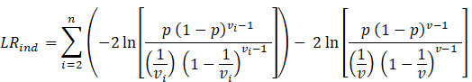
Haas (2001) developed a back test that considers the time between successive failures. He takes advantage of the TUFF test to measure the time in-between failures and combines with the POF test to check if the overall rate of failure is accurate. Haas proposes the following test statistic:

 

 

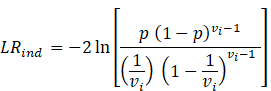
where  represents the time interval between two exceptions. Hence, a test statistic must be calculated for each exception. By combining the different likelihood-ratios, one gets  :

 

 

which is also chi-squared distributed, with n degree of freedom. Adding it with the POF test, we get our mixed test. The likelihood ratio is,

 

 

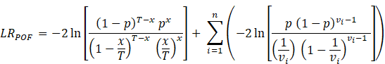
 is also chi-squared distributed with n+1 degree of freedom.

 

4. CONCLUSION

In this monograph, we have calculated VaR of NIFTY 50 with four approaches. Approaches used are variance covariance method, historical simulation, a Monte Carlo simulation, and cubic polynomial regression method. The VaR estimates back-testing is discussed with total exception check, Basels’ Traffic light zone test, Kupiec’s POF-test, Kupiec TUFF-test, and Haas’ Mixed-Kupiec-test.

We observed that in calm market conditions all back testing approaches approves the VaR model performance. Monte-Carlo simulation and Cubic polynomial regression method works better compared to historical simulation and parametric approach. In highly volatile market conditions such as financial crises all four VaR models have weak performance according to back-testing results.

Based on this case study of Nifty 50 over 2834 days of data. we indicated that VaR model should be used for corresponding requirements if clustering of failures is of interest Kupiec TUFF-test and Mixed Haas Kupiec tests better validate the VaR model. If overall failures are of interest, then Total exceptions, Kupiec POF-test are good for validation of VaR model. If one is interested in reducing failures in overestimation and underestimation cases one can opt for Basels’ traffic light zone test.

For our case study of four methods of VaR using different back testing approaches on NIFTY 50 index, we observed that all four VaR method performs well for 95 % confidence interval. For 99% or higher confidence level all methods are rejected by back-testing approaches.

We also conclude that back-testing period should be of appropriate size two to three years to avoid the clustering of exceptions and volatility effects.

 

CONFLICT OF INTERESTS

None. 

 

ACKNOWLEDGMENTS

None.

 

REFERENCES

Abad, P., Benito, S., and López, C. (2014). A Comprehensive Review of Value at Risk Methodologies. The Spanish Review f Financial Economics, 12(1), 15-32. https://doi.org/10.1016/j.srfe.2013.06.001.

BCBS. (1996).

Dowd, K. (1998). Beyond Value at Risk : The New Science of Risk Management. Wiley, New York.

Glasserman, P. (2004). Monte Carlo Methods in Financial Engineering. New York : Springer.  53, Xiv+-596.

Gupta, M., Vaniya, K., and Gor, R. (2021). Review on Var Using Monte-Carlo Simulation, EWMA and GARCH Models. Proceedings of International Conference on Mathematical Modelling and Simulation in Physical Sciences (MMSPS-2021). Excellent Publishers, 332-337.

Gustafsson, M., and Lundberg, C. (2009). An Empirical Evaluation of Value at Risk.

Haas, M. (2001). New Methods In Backtesting. Financial Engineering Research Center, Bonn.

Morgan, J.P.  (1994). "RiskMetrices-Technical Document".

Jackson, P., Maude, D., and Perraudin, W., (1998). Bank Capital and Value-at-Risk. Bank of England. Bank of England Quarterly Bulletin, 258-266. https://doi.org/10.2139/ssrn.87288.

Jascha Andri Forster (2015). "Backtesting of Monte Carlo value at risk simulation based on EWMA volatility forecasting and cholesky decomposition of asset correlations".

Jondeau, E., and Rockinger, N.(2003). Conditional Volatility, Skewness and Kurtosis : Existence, Persistence, and Comovements. Journal of Economic Dynamics and Control, 27, 1699-1737. https://doi.org/10.1016/S0165-1889(02)00079-9.

Jorion, P. (1996). Risk 2 : Measuring the Risk in Value at Risk. Financial Analysts Journal, 52(6), 47-56. https://doi.org/10.2469/faj.v52.n6.2039.

Jorion, P. (2007). Value at Risk : The New Benchmark for Managing Financial Risk, Mcgraw-Hill New York.

Katsiampa, P. (2017). Volatility Estimation for Bitcoin : A Comparison of GARCH Models. Economics Letters, 158, 3-6. https://doi.org/10.1016/j.econlet.2017.06.023.

Kupiec, J., Pedersen, J., and Chen, F. (1995). A Trainable Document Summarizer. In Proceedings of the 18th Annual International ACM SIGIR Conference on Research and Development in Information Retrieval, 68-73. https://doi.org/10.1145/215206.215333.

Kupiec, P. H. (1995). Techniques for Verifying the Accuracy of Risk Measurement Models. Division of Research and Statistics, Division of Monetary Affairs, Federal Reserve Board. 95(24). https://doi.org/10.3905/jod.1995.407942.

MBA in Business Finance.

Morgan, J. P. (1996). Creditmetrics-Technical Document. JP Morgan, New York. Creditmetrics-Technical Document

Naimy, V., Chidiac, J. E. and Khoury, R. E. (2020). Volatility and Value at Risk of Crypto Versus Fiat Currencies. In International Conference on Business Information Systems, Springer, Cham.,145-157. https://doi.org/10.1007/978-3-030-61146-0_12.

Nieppola, O. (2009). Backtesting Value-at-Risk Models.

Raaji, G. and Raunig, B. (1998). A Comparison of Value at Risk Approaches and Their Implications for Regulators. Focus on Austria, 4, 57-71.

Rajput, S. and Vaniya, K. (2021). Value at Risk (Var) Calculation Using Parametric Methods and Optimization. Proceedings of International Conference on Mathematical Modelling and Simulation In Physical Sciences (MMSPS-2021), Excellent Publishers. 338-342.

Vaniya, K. and Gor, R. (2020). Computation of Value at Risk (Var) Using Cubic Polynomial Fitting Approach. Alochana Chakra Journal, 3832-3846.

Vaniya, K. and Gor, R. (2021). Computation of Var Using Continuous Curve Fitting Approach. PIMT Journal of Research, July-Sept., 13(4), 159-164.

Vaniya, K. and Gor, R. (2022). VaR and CVaR of Indian Stocks Using Simulation Model and Back Testing. IOSR Journal of Economics and Finance (IOSR-JEF), 13(02), 60-69.

Vaniya, K., Talaviya, R., and Gor, R. (2022). Estimating Value at Risk Using Monte-Carlo Simulation. IOSR Journal of Mathematics (IOSR-JM), 18(4), 16-23.

Vaniya, K., and Gor, R. (2021). VaR and CVaR Using Monte-Carlo Simulation and Cubic Polynomial Fitting Approch. Proceedings of International Conference on Mathematical Modelling and Simulation in Physical Sciences (MMSPS-2021), Excellent Publishers, 299-305.

Yawalkar, P. G., and Rao, P. (2004). Backtesting of Value at Risk (Var) Methods for Fixed Income Security (FIS) and Equity Portfolios in Indian Market Conditions.