APPLICATION OF FIRST-ORDER DIFFERENTIAL EQUATIONS

 

G. Mahata ¹ , D.S Raut ¹, C. Parida ¹, S. Baral ¹, S. Mandangi ¹

 

¹ Department of Mathematics C. V. Raman College of Engineering, Bhubaneswar-752054, India

 

1. INTRODUCTION

The equation contains one or more than one derivative is known as differential equations or in other words we can say the equation that contain derivative of one or more dependent variable with respect to one or more independent variables. Differential equations have remarkable ability to predict the world around us. They are used in a wide variety of disciplines, from biology, economics, chemistry, and engineering. The differential equation which contains only first order derivative is known as first order differential equation. Basically, we divide differential equation into two categories that are ordinary differential equation and partial differential equation. The ordinary differential equation contains unknown functions of one independent variable whereas the partial differential equation contains unknown function of more than one independent variable. We discussed more about this further in this paper. In this paper we are going to discussed about first order differential equations and its solution and its application to heat convection in fluid.

First order differential equation has a lot of application in the area of heat transfer which is discovered by Karthikeyan and Srinivasan Hassan and Zakari (2018). Also, the first order differential equation has many applications in temperature problem basically the ordinary differential equation. From which Hassan and Zakari Karthikeyan and Jayaraja (2016) found the use of newton’s law of cooling in solving some practical problem of first order ordinary differential equations. Mahanta et al. (2015, 2016) carried the analysis convective boundary condition. Rehan Hsu (2018) studied the first order differential equations and newtons law of cooling. Keryzig Rehan (2020), Caronongan Hsu (n.d.),        Michael Keryszig (2006). carried the solution of first order and applications of differential equations has been considerd.

 

2. TYPES OF DIFFERENTIAL EQUATION

· Ordinary differential equations

The equations where the derivatives are taken with respect to only one variable is known as ordinary differential equations.

For e. g. dy/dx = sinx

· Partial differential equations

The equation in which one variable depends on more than one variable is known as partial differential equations.

For e. g.

· Linear differential equations

The linear differential equation is of the form dy/dx+p(x)y=Q(x)

· Non-linear differential equations

A non-linear differential equation that is not a linear equation in the unknown function and its derivatives.

It is of the form

· Homogeneous and non-homogeneous differential equations

A homogeneous equation does have zero on the right side of the equality while a non-homogeneous equations have a function on right side of the equations.

For e. g.  (homogeneous differential equation)

                 (non-homogeneous differential equation)

Now our main focus is on solutions of first order differential equation and its application

 

3. Solution of first order differential equations

1)    Using integrating factor

 The linear differential equation is of the form

 

                    

 

Then the integrating factor is defined by the formula

 

IF =            

        

 Then the general solution is

 

                                   Y =

 

2)    Method of variation of a constant

This method is similar to integrating factor method. finding the general solution of the homogeneous equation is the first necessary step.

 The homogeneous equation is

 

                                                           

 

The general solution of the homogeneous equation always contains a constant C. The value of C we get after substituting the solution into the non-homogeneous differential equation. This method is known as method of variation of a constant.

 

NOTE

The solution in both of above method is always same.

Problem 1

    Solve the differential equation

  Solution

 The given equation is already in a standard form,

    

    Therefore p(x)= 2x and q(x)= x

     Now IF=

     Now Y(x)=  =

 

· Application of first-order differential equation to heat convection in fluid

1)    Heat transferring

Heat transferring is a process of transfer of heat from a body with higher temperature to a body with lower temperature. Hear the difference between the temperature is called potential for which transfer of heat is happen. There is different mode for heat transferring which are as follow

· Conduction

· Convection

· Radiation

 

 

 

 

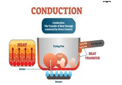
1)    Conduction

The process by which the heat is transfer from hot end of an object to its cold end is called conduction. It is also known as thermal conduction or heat conduction. Basically, in solid heat is transferred by the process of conduction.

Figure 1

Figure 1

 

2)    Convection

The process by which fluid molecules moves from higher temperature region to lower temperature region is called convection.

Figure 2

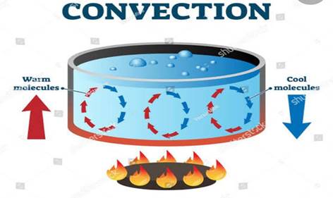
Figure 2

 

3)    Radiation

Radiation is the transfer of energy with the help of electromagnetic wave. It is generated by the emission of electromagnetic wave.

Figure 3

 

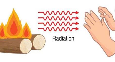
Figure 3

 

So above we have seen that heat flowing in solid by the process of conduction which we can determined by Fourier law. And we see in fluid, heat flowing by convection which we can determine by Newton’s law of cooling.

 

NEWTON’S LAW OF COOLING

 Statement

              Let Q= heat absorbed

                    T =temperature of the body

                    =surrounding temperature

Newton’s law of cooling state that the temperature of the body and its surrounding is directly proportional to the rate of cooling of the body.

 

 i.e.                                                                                                                       (1)

   

    or dQ = h [

 

   Now integrating on both sides, we get

 

Hear ,  so heat transform from

Again, for a body of mass ‘M’, specific heat ‘’, temperature of the body ‘T’  kept in surrounding temperature ‘’

Then, heat = mass*specific heat*body temperature

 

I. e. Q = M

 

Now rate of colling is given by

         

Hence, we found that

           

Due to specific heat and mass of the body treated as constant so,

Hence the above explanation suggested that as the time increases the difference between the body temperature and surrounding temperature increases so that the rate of temperature decreases.

 

Problem 2

A body cools from 75 to 55 in 10 minutes when the surrounding temperature is 31. At what average temperature will its rate of cooling be ¼ to that at the start.

Solution

        Let  be the temperature of the surrounding

        Consider a colling from

Initial temperature =  =

Final temperature =

Time taken t = 10 min

 

We know

 

      

 

Consider the rate of cooling when the temperature was

Rate of cooling  = ¼

Now

 

       

     

   

   

   

 

Hence at temperature 39.5 the rate of cooling be ¼th that at the start.

 

Problem 3

   A heated metal ball is placed in cooler surroundings. Its rate of cooling is 2 per minute when its temperature is 60 and 1.2 per minute when its temperature is 52. Find the temperature of the surroundings and the rate of cooling when the temperature of the ball is 48.

Solution

        Let  b e the temperature of the surrounding

Consider a cooling at 60:

   Temperature = 60

    Rate of cooling = 2 per minute

  By newton’s law of cooling,

 

              

                                                                                                             (1)

 

Consider a cooling at 52:

    Temperature =52

     Rate of cooling = 1.2 per minute

Again, by newton’s law of cooling,

 

             

                                                                                                          (2)

 

Now dividing equation (1) by (2) we get,

 

            

     

      

      

 

Substituting in equation (2) we get,

 

       1.2 = h (52-40)

 

 

To find rate of cooling at 48:

 By newton’s law of cooling,

 

          

     

     

 

Hence temperature of the surrounding is 40 and rate of cooling at 48 is 0.8  per minute.

 

Application of first order differential equation: Orthogonal trajectory

Before going to know what, orthogonal trajectory is, we have to know trajectory first.

·        Trajectory

A curve which cut every member of a given family of curve is called trajectory.

Figure 4

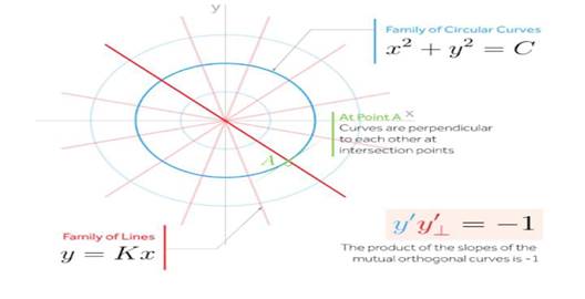
Figure 4

 

·        Orthogonal trajectory

A curve which cuts every member of a family of curve at right angle is called orthogonal trajectory. Or in other words it is the family of curve that intersect perpendicularly to another family of curve.

Mathematically,

If we have a family of curve given by F(x,y,a) = 0 and another family of curve   G(x,y,b). then the tangent of the curve is perpendicular to each other. Where a and b are arbitrary constant.

          Orthogonal trajectories are used in mathematics for example as curve coordinate system or appear in physics as electric field and its equipotential curve.

 

Step to find orthogonal trajectory:

Case 1- for cartesian curve

1)     Differentiate the given equation of family of curve and eliminate the parameter

2)     Replace

3)     Solve the new differential equation and get orthogonal trajectory.

 

Case – 2      for polar curve

1)     Differentiate the given equation of family of curve with respect to .

2)     Replace

3)     Solve new differential equation and get required solution            

 

Problem 4

Find the orthogonal trajectory of .

Solution

        Given curve, 

        Differentiate the given equation w.r.t x

        

   

  

  

  

Integrating on both the side

  

 

 

Hence, the orthogonal trajectory of

 

Problem 5

Find the orthogonal trajectory of family of parabola

Solution

Given

Differentiate both the side w.r.t x

 

  

 

   Putting the value of a in the given equation of curve we get,

  

                                                                                                   (1)

 

 

   

     

This equation is same as equation (1), so if we integrate this, we get the given curve

Hence the orthogonal trajectory of is itself.

 

Problem 6

Find the orthogonal trajectory of cardio’s

Solution

Given

Differentiate both the side w.r.t

 

 

Eliminate a from given equation

 

    

   

  

  

  

Integrating on both side

 

 

 

 

 

  , where b = c/2

Hence r = b (1+cos θ) is the orthogonal trajectory of r = a(1-cos θ)

 

4.  Conclusion

In this paper we discussed applications of first order differential equation that is newtons law of cooling and orthogonal trajectory. Newton’s law of cooling states that the rate at which an objects cools is directly proportional to the difference in temperature between the object and its surrounding. It explains how fast an object is cool down. However, it works only if the difference in temperature between body and its surrounding must be small, the loss of heat from the body should be by radiation only. And the major limitation of newtons law of cooling is that the temperature of the surrounding must remain constant during the cooling of the body.

Whereas orthogonal trajectory is the tangent of two curve which are perpendicular to each other.  Here we see the use of first order differential equation which allow these variables to be expressed dynamically as a differential equation for the unknown position of the body as a function of time. It has a major role in forensic science. The are many such application of first order differential equation such as population growth and decay, drug distribution in human body, survivability with AIDS, radioactive decay and carbon dating, economics, and finance etc. finally this paper believed that many problems of science and technology in future can be solve by using first order differential equation.

 

CONFLICT OF INTERESTS

None. 

 

ACKNOWLEDGMENTS

None.

 

REFERENCES

Caronongan, k. (2010). An Application Differential Equation in the study of Elastic columns, Research Paper, Paper 5.

George F. Simmons (2017). Differential Equation with Application and Historical notes, 3rd ed. Chapman and Hall/crc.

Hassan, a. and Zakari, y. (2018). Application of First Order Differential Equation in Temperature Problem.

Karthikeyan, N. and jayaraja, A. (2016). Application of First Order Differential Equation to Heat Transferring in Solid.

Keryszig, E (2006). Advance Engineering Mathematics.9th edition, willey, India

MATH24 (2022).

Mahanta, G, Shaw, S. (2015). 3D Casson Fluid Flow Past a Porous Linearly Stretching Sheet with Convective Boundary Condition. Alexandria Engineering journal, 54(3), 653-659. https://doi.org/10.1016/j.aej.2015.04.014

Mahanta, G.Shaw, S. (2015). Soret and Dufour Effects on Unsteady MHD Free Convection Flow of Casson Fluid Past a Vertical Embedded in a Porous Medium with Convective Boundary Conditions. International Journal of Applied Engineering Research, 10 (10), 24917-24936.

Rehan, Z. (2020). Applications of First Order Differential Equations to Heat Convection in a Fluid. Journal of Applied Mathematics And Physics, 8, 1456-1462. https://doi.org/10.4236/jamp.2020.88111

Shaw, S. Mahanta, G.P, Sibanda (2016). Non-Linear Thermal Convection in a Casson Fluid Flow Over a Horizontal Plate with Convective Boundary Conditions, 55(2), 1295-1304. https://doi.org/10.1016/j.aej.2016.04.020

Stack Exchange (2022).

Tai-Ran Hsu (2018). Applications of First Order Differential Equations in Engineering Analysis, Applied Engineering Analysis.

Tai-Ran Hsu (n.d.). Application of First Differential Equation in Mechanical Engineering Analysis