ARIMA MODEL FOR FORECASTING THE BITCOIN EXCHANGE RATE AGAINST THE USD

 

Vasantha Vinayakamoorthi ¹, Saravanamutthu Jeyarajah ²,  Jeyapraba Suresh ² , Niroshanth Sathasivam ³

 

¹ Lecturer, Department of Economics, Eastern University Sri Lanka, Eastern Province, Sri Lanka

² Senior Lecturer, Department of Economics, Eastern University Sri Lanka, Eastern Province, Sri Lanka

³ Department of Software Technology, University of Vocational Technology, Sri Lanka

1. INTRODUCTION

Currently, the most popular digital currency is bitcoin. Bitcoin's recognition as a valuable investment asset is on the rise. A peer-to-peer, completely decentralized cryptocurrency system called BTC was created to enable online users to perform transactions using virtual money known as bitcoins. It is decentralized because it is neither governed nor managed by a single organization Ayaz et al. (2020).

A prediction method is required to assist its customers in forecasting the price in the future in order to deal with the unpredictable changes in the price of bitcoin Wirawan et al. (2019). It has received a lot of attention recently in a variety of domains, such as computer science, economics, and finance. If we had the ability to sell our assets ahead of a price crash and then buy them again when prices fell. In order to anticipate the price of Bitcoin in the future, we employed a time series forecasting method called ARIMA. The results were quite intriguing.

There is a need to research ways to comprehend Bitcoin's price changes given that it is growing in popularity while yet remaining unpredictable and little understood. Making accurate daily predictions can boost day traders' profits and, as a result, improve the market's efficiency. Performance can be significantly impacted by the model selection for predicting Chen et al. (2019).

Most of the related studies find the ARIMA model before the pandemic of covid. Very few studies consider the forecasting concept through the ARIMA model. Current two years also, the BTC exchange rate dramatically increased to the top. At the same time, it faced a decreased pattern nowadays. Many countries consider cryptocurrency for their economic development.  So, we want to identify the shootable model for forecasting to predict the exchange rate of BTC. This study finds out 2 objectives. The first one is to identify the best ARIMA model for forecasting. The Second object is to predict the next 5-month bitcoin exchange rate against the USD.

 

2. LITERATURE REVIEW

Wirawan et al. (2019) Investigate the Short-term prediction of Bitcoin price using the ARIMA method. The Autoregressive Integrated Moving Average (ARIMA) approach is used to make predictions and may produce short-term predictions with a high degree of accuracy. Use of Mean Absolute Percentage Error to Analyze Prediction Results (MAPE). According to the findings, ARIMA (4,1,4) models produced predictions with the minimum MAPE, 0.87 for the following one-day projection and 5.98 for the following seven days. As a result, it is possible to anticipate Bitcoin prices for the next one to seven days using the ARIMA (4,1,4) model.

Dhinakaran et al. (2022) demonstrate, through an analysis of the price time series over a three-year period, the benefits of the conventional Autoregressive Integrative Moving Average (ARIMA) model in predicting the future value of cryptocurrencies. On the one hand, empirical studies demonstrate that the behaviour of the time series is essentially unchanged; on the other hand, when used for short-term prediction, this straightforward method is largely effective in sub-periods. A further investigation in cryptocurrency price prediction using an ARIMA model trained over the entire dataset is discussed below.

Bakar and Rosbi (2017) examined ARIMA Model for Forecasting Cryptocurrency Exchange Rate. The parameter of the ARIMA model was determined by this study's examination of the autocorrelation function (ACF) and partial autocorrelation function (PACF). As a result, the first variation in the price of a bitcoin is a stationary data series. ARIMA was used as the forecasting model in this investigation (2, 1, 2). The informational Akaike criterion is 13.7805. This model is regarded as having good fitness. Ex-post forecasting has a mean absolute percentage error of 5.36 percentage based on the error analysis between the predicted value and actual data. The results of this study will help forecast the price of bitcoin in an environment with high volatility.

Based on a time series analysis method known as the autoregressive integrated moving average (ARIMA) model, Vidyulatha et al. (2020) research is conducted on five and a half years' worth of bitcoin data from 2015 to 2020. Additionally, the linear regression (LR) model, an existing machine learning approach, is also contrasted. The suggested ARIMA model outperformed the LR model in terms of short-term volatility in weighted bitcoin costs, according to extensive prediction findings.

To forecast Bitcoin's log returns, Kim et al. (2022) used linear and nonlinear error-correcting models (ECMs) (BTC). In terms of RMSE, MAE, and MAPE, the linear ECM outperforms the neural network and autoregressive models at predicting BTC. We can comprehend how other coins affect BTC by using a linear ECM. In addition, we tested fourteen cryptocurrencies for Granger causality.

 

3. RESEARCH METHODOLOGY

3.1.  DATA SELECTION

From January 2015 through June 2022, monthly data for the exchange rate of bitcoin were chosen for this study. The information is gathered from https://www.investing.com.

 

3.2. BOX-JENKINS ARIMA MODEL

Forecasting is the process of speculating about what will happen in the future. Due to the uncertainty, a forecast's accuracy is just as crucial as the result it predicts. There are three classifications of widely used forecasting techniques.  

Figure 1

                                                                     

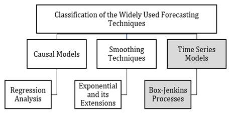
Figure 1 Classification of Forecasting Techniques

 

The Autoregressive Integrated Moving Average Model (also known as ARIMA) is a widely used statistical model for forecasting and analysing time data. The authors’ Box and Jenkins also propose a procedure for selecting, estimating, and verifying ARIMA models for a particular time series dataset.

The first step is to make the plot of the series. Then check whether the variance is stationary or not. If the variance is non-stationary, will apply the shootable transformation method and otherwise check whether the mean is stationary or not. if the mean is non-stationary, will apply the regular and seasonal differencing to the data. After making the stationary series, identify the model selection. Every time check whether the residual parameters value correlated or not. if is it ok the series is, next we want to check the significant level of parameters. If that model is adequate, we will check the diagnostic test to confirm the validity of the fitted model. Finally, we can forecast the particular data.

 

3.3. ACF and PACF

The correlation between observations of a time series that are separated by k time units ( is measured by the autocorrelation function. To find ARIMA models, combine the partial autocorrelation function with the autocorrelation function. Check to see if any of the spikes at each lag are substantial. The significance thresholds will be exceeded by a significant spike, proving that the correlation for that lag isn't equal to zero.

 

3.4. NORMALITY, BOX-COX TRANSFORMATION AND REGULAR AND SEASONAL DIFFERENCE

The data collection may follow a normal distribution if you do a straightforward computation called a Box-Cox Transformation. George Box and Sir David Cox, two British statisticians, are credited with creating the Box-Cox transformation.

To determine if the data follows a normal distribution or not, use the normality test. the null and alternative hypotheses are given below.

 Data follow normal Distribution

 Data does not follow a normal distribution

Then will do the step to transform the data using Box-Cox transformation. After that conclude or select the shoutable transformation method through the below criteria. Table 1

Table 1

Table 1  Value and Transform data
(Rounded Value)	Transform Data
-2
-1
-0.5
0
0.5
1
2

 

ARIMA models can also be used to model a variety of seasonal data. By incorporating additional seasonal components into the ARIMA models we have seen thus far, a seasonal ARIMA model is created. It reads as follows.

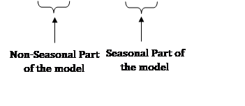
Where,

p, P – AR Part

q, Q – MA Part

d, D – Integration

m – Number of observations per year

The seasonal lags of the PACF and ACF will show the seasonal component of an AR or MA model. An example of a representation of a random process is an autoregressive (AR) model. In time series data, it is used to describe some time-varying processes. According to the moving-average model, the output variable is linearly dependent on the present value as well as various previous values of a stochastic (Imperfectly predictable) factor.

 

3.5. MODEL SELECTION CRITERIA

Even while one model may occasionally be appropriate for any given collection of data, the accuracy of a forecasting model necessitates that a number of models are compared in order to determine which one yields the best results with the fewest errors. The mean squared error of all forecasts, or MSE, is the initial evaluation criterion.

 

 

Where,

 - The i^th observed value

 - The corresponding predicted value

n - The number of observations

 

4. RESULTS AND DISCUSSION

4.1. DATA DESCRIPTION

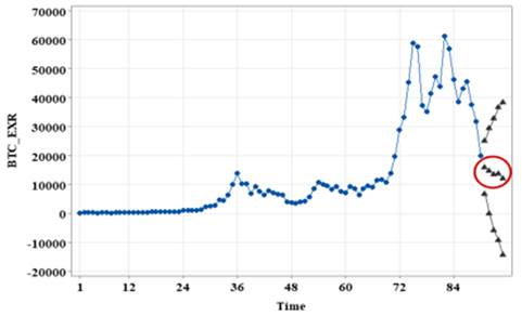
The Bitcoin exchange rate against the USD is shown in Figure 2. The chosen observational data span the period of time from January 2015 to June 2022. There have been 90 observations in total.

Figure 2

                                                                     

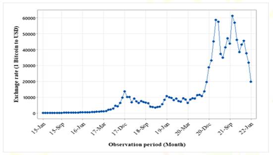
Figure 2 Bitcoin Exchange Rate Against USD (Monthly Data from Jan-2015 To Jun-2022)

 

From January 2015 to August 2020 Bitcoin exchange rate against the USD slowly increased. In September 2020, the Bitcoin exchange rate against the USD dramatically increased up to March 2021. Increased demand from institutional and retail investors who viewed the virtual currency as a shelter and an inflation hedge has contributed to this growth. Then it decreased with fluctuated. The minimum and maximum values of the Bitcoin exchange rate against the USD are 217 and 61330. It is shown in Table 2.  

Table 2

Table 2 Basic Statistics
Variable	N	Mean	Median	Minimum	Maximum
BTC_EXR (Bitcoin exchange rate against USD)	90	12946	6976	217	61330

 

4.2. STATIONARY TEST AT LEVEL FORM

Figure 3

                                                                     

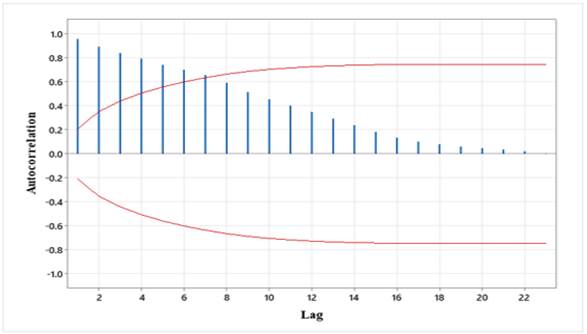
Figure 3 Autocorrelation Function (ACF) For BTC_EXR (With 5% Significance Limits for the Autocorrelations)

 

According to the ACF, there is slow decay in autocorrelation analysis. Therefore, exchange rate data is non-stationary data. Otherwise, conclude it is non-stationary with mean and variance.

 

4.3. NORMALITY TEST AND DATA TRANSFORMATION

According to the Normality test Figure 4, the p-value (0.005) is less than the alpha value (0.05). Thus accept the alternative hypothesis. So, the data are not normally distributed.

 

 

 

Figure 4

                                                                     

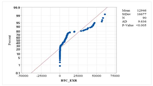
Figure 4 Normality Test

 

Then choose the shoutable transformation to the data. According to the Box-Cox Transformation method, the rounded value is 0.  So, the shootable transformation is a log transformation. It was clearly shown in Figure 5.

Figure 5

                                                                    

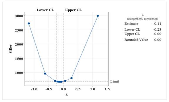
Figure 5 Box-Cox Plot of BTC_EXR

 

4.4. STATIONARY TEST AT LOG FORM

According to Figure 6 and Figure 7, we can conclude the data is non-stationary still with the mean. Because the initial spikes follow the decay.

 

 

Figure 6

                                                                     

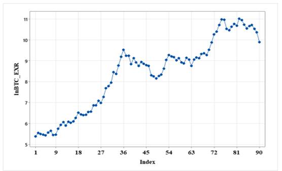
Figure 6 Time Series Plot of ln BTC_EXR

 

Figure 7

                                                                     

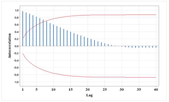
Figure 7 Autocorrelation Function (ACF) for ln BTC_EXR (with 5% significance limits for the autocorrelations)

 

4.5. SEASONALITY ADJUSTMENT BY DIFFERENCING

Stationery needs to be created for the series. Therefore, using the log function to modify the data, we must remove the trend and seasonality from the series to make it stationary. As seen in Figure 6, the results are unsatisfactory, thus we must apply seasonal and regular differencing, one of the most popular techniques for dealing with both trend and seasonality. Figure 8, Figure 9, Figure 10.

 

Figure 8

                                                                     

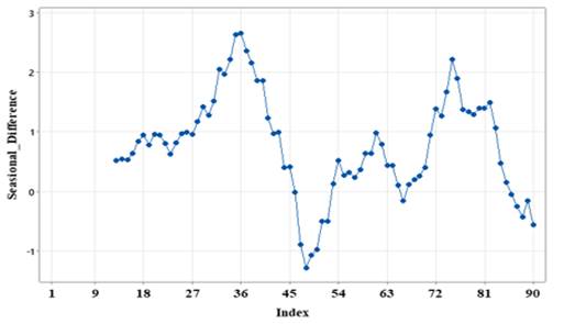
Figure 8 Time Series Plot of Seasional Difference

 

Figure 9

                                                                     

Figure 9 Autocorrelation Function (ACF) for Seasional_Difference (with 5% significance limits for the autocorrelations)

 

Figure 10

                                                                      

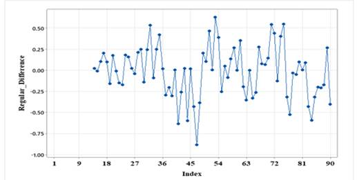
Figure 10 Time Series Plot of Regular Difference

 

Visually, we can see time series have been made stationary at this point. The next step is to use ARIMA to create a model on the time series. We must first determine the values of the parameters p, q, and d before we can implement the ARIMA function.

 

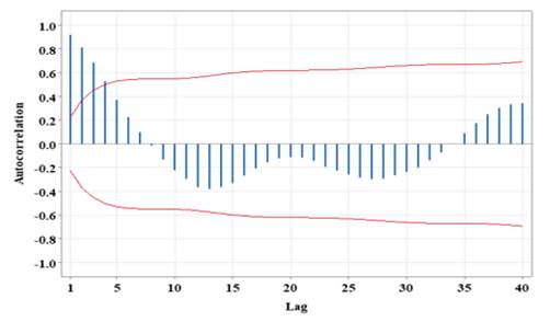
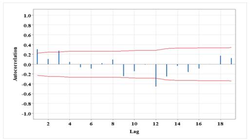
4.6. PARAMETER ESTIMATION FOR ARIMA

Two charts, the Autocorrelation Function (ACF) - Minitab. (N.D.) and the Partial Autocorrelation Function are used to calculate the values of "p" and "q." (PACF). Figure 11, Figure 12.

Figure 11

                                                                     

Figure 11 Autocorrelation Function (ACF) - Minitab. (N.D.) for Regular difference with a seasonal difference (with 5% significance limits for the autocorrelations) – MA part

 

Figure 12

                                                                     

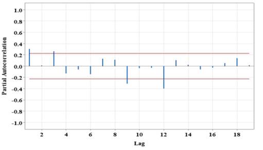
Figure 12 Partial Autocorrelation Function (ACF) for Regular difference with a seasonal difference (with 5% significance limits for the partial autocorrelations) – AR part

 

We have used the ARIMA technique to model time series in order to predict the Bitcoin exchange rate against the USD. The best models are thought to have a lower MSE. To determine the best fit for our model, we experimented with a variety of ARIMA combinations in an effort to attain a lower MSE value. According to Table 2, The forecast model implemented in this study is ARIMA . Comparing other ARIMA models, our fitted model is lower MSE, and 5 significant value is there. The fitted model predicted parameters’ (5 Parameters) probability value is less than the alpha value (0.05). Thus, All the variables are stationary.  According to the Ljung-Box chi-square statistics, 12,24,36,48 lags’ probability values are greater than the alpha value (0.05). So, The Modified Box-Pierce test suggested that there is no autocorrelation left in the residuals. This model is considered a model with good fitness.  

Table 3

Table 3 Summary Table of ARIMA Combinations
ARIMA Model	Final Estimates of Parameters (Significant values)	MSE	Ljung-Box Chi-square Statistics (Significant lag)
	2	0.0614806	12,24,36,48
	3	0.0455948	12,24,36,48
	4	0.0449887	12,24,48
	4	0.0414699	12,24,36,48
	5	0.040462	12,24,36,48

 

Table 4

Table 4 Predicted model Parameters Estimation -
Type	Coef	SE Coef	P-Value
AR 1	0.265	0.121	0.032
SAR 12	-0.344	0.15	0.025
SAR 24	0.398	0.156	0.013
SMA 12	0.799	0.159	0
Constant	-0.02178	0.0055	0

 

Table 5

Table 5 Modified Box-Pierce (Ljung-Box) Chi-Square Statistics
Lag	12	24	36	48
Chi square	5.67	19.49	30.63	48.30
DF	7	19	31	43
P-Value	0.579	0.426	0.485	0.267

 

4.7. NORMALITY TEST FOR RESIDUAL CHECKING TO ARIMA

According to the output of Normality test for residual, the probability value is 0.890. It was higher than the alpha value (0.05). S we accept the null hypothesis. Thus, we can say the residual series is Normally distributed in our fitted model. It was indicated in the Figure 13.

Figure 13

                                                                      

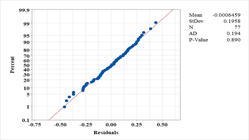
Figure 13 Normality Test for Residual

 

4.8. DIAGNOSTIC TEST

Figure 14

                                                                    

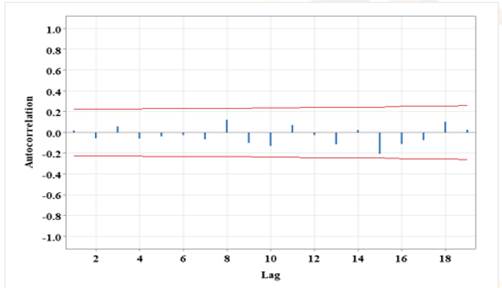
Figure 14 ACF for Residual (with 5% significance limits for the autocorrelations)

 

Figure 15

                                                                     

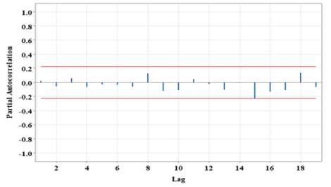
Figure 15 PACF for Residual (with 5% significance limits for the partial autocorrelations)

 

4.9. FORECASTING

Finally, we are going to predict the Bitcoin exchange rate against the USD from July 2022 to November 2022. Figure 13 displays the plot for the Bitcoin exchange rate against the USD over the next five months after an ARIMA model was fitted to the time series data.

Table 6

Table 6 Forecasting Values
Period	Forecast	95% Limits
		Lower	Upper
Jul-22	15834.6	6668.6	25000.7
Aug – 2022	14562.9	-303	29428.7
Sep – 2022	13347.9	-6014.6	32710.5
Oct – 2022	13635	-9466.7	36736.7
Nov-22	11968.3	-14372.3	38308.9

 

Figure 16

                                                                    

Figure 16 Plot of Forecasting Values (Jul – 2022 to Nov – 2022)

 

5. CONCLUSION AND RECOMMENDATION

In this study, we have investigated the bitcoin exchange rate against the USD prediction by using the ARIMA model (. Log transformed method was used to make the stationary with variance and also apply the regular and seasonal difference to make the stationary with mean. In the best adequate model, all parameters are stationary. The predicted model also fitted well. This study only considers the bitcoin exchange rate against the USD. In the cryptocurrency market, the lead coin is BTC. But also, there are so many altcoins. So, except for the BTC, Investors or analysts need to consider the forecasting area. A reliable forecasting model is produced by the forecasting strategy employing the autoregressive integrated moving average (ARIMA) method. Error diagnostics must be given extra consideration while forecasting in high volatility environments. Investors will be able to forecast the future bitcoin exchange rate against the USD with the aid of this information.

 

CONFLICT OF INTERESTS

None. 

 

ACKNOWLEDGMENTS

No specific grant was given to this research by any funding organization in the public, private, or non-profit sectors.

 

REFERENCES

Autocorrelation Function (ACF) - Minitab. (N.D.). Autocorrelation Function (ACF) - Minitab, Support.Minitab.Com.

Ayaz, Z., Fiaidhi, J., Sabah, A., And Ansari, M. (2020). Bitcoin Price Prediction Using ARIMA Model. https://doi.org/10.36227/techrxiv.12098067.v1.

BTC USD Bitfinex Historical Data - Investing.Com. (N.D.). Investing.Com.  

Bakar, N. A. and Rosbi, S. (2017). Autoregressive Integrated Moving Average (ARIMA) Model for Forecasting Cryptocurrency Exchange Rate in High Volatility Environment : A New Insight of Bitcoin Transaction, International Journal of Advanced Engineering Research and Science, 4(11),130-137. https://dx.doi.org/10.22161/ijaers.4.11.20.

Chen, A.S., Chang,H. C., And  Cheng, L.Y. (2019). Time-Varying Variance Scaling: Application of the Fractionally Integrated ARMA Model. The North American Journal of Economics and Finance, 47, 1–12. https://doi.org/10.1016/j.najef.2018.11.007.

Dhinakaran, K., Baby Shamini, P., Divya, J., Indhumathi, C. and Asha, R. (2022). "Cryptocurrency Exchange Rate Prediction Using ARIMA Model on Real Time Data," 2022 International Conference on Electronics and Renewable Systems (ICEARS), 914-917, https://doi.org/10.1109/ICEARS53579.2022.9751925.  

Frost, J. (2021). Mean Squared Error (MSE) - Statistics by Jim. Statistics by Jim, Statisticsbyjim.Com.  

Gertrude Chavez-Dreyfuss, T. W. (N.D.). Bitcoin Surges to All-Time Record as 2020 Rally Powers on, Reuters. U. S.

Hessing, T., and PV, R. (2014). Box Cox Transformation. Six Sigma Study Guide, Sixsigmastudyguide.Com.  

Kim, J. M., Cho, C. and Jun, C. (2022). "Forecasting the Price of the Cryptocurrency Using Linear and Nonlinear Error Correction Model". Journal of Risk and Financial Management, 15(2), 74. https://doi.org/10.3390/jrfm15020074. 

Seasonal ARIMA Models (2022). Forecasting : Principles and Practice (2nd Ed). (N.D.). 8.9 Seasonal ARIMA Models. Forecasting: Principles and Practice (2nd Ed), Otexts.Com.     

Specify a Box-Cox Transformation for Individual Distribution Identification - Minitab. (N.D.). Specify a Box-Cox Transformation for Individual Distribution Identification - Minitab, Support.Minitab.Com.

Time-Critical Decision Modeling and Analysis. (N.D.). Home.Ubalt. Edu.

Tularam, G. A., and Saeed, T. (2016). Oil-Price Forecasting Based on Various Univariate Time-Series Models. American Journal of Operations Research, 6(3), 226–235. https://doi.org/10.4236/AJOR.2016.63023.   

Vidyulatha, G., Mounika, M., And Arpitha,N. (2020). Crypto Currency Prediction Model Using ARIMA, Turkish Journal of Computer and Mathematics Education, 11(3), 1654 – 1660.

Wirawan, M., Widiyaningtyas, T. and Hasan, M. M. (2019)."Short Term Prediction on Bitcoin Price Using ARIMA Method," 2019 International Seminar on Application for Technology of Information And Communication (Isemantic), 2019, 260-265. https://doi.org/10.1109/ISEMANTIC.2019.8884257.

     

APPENDICES

  Appendix 1

Appendix 1 “APPENDIX A,”
Month	BTC_EXR	lnBTC_EXR
15-Jan	217.4	5.3817
15-Feb	255.7	5.544
15-Mar	244.3	5.4984
15-Apr	236.1	5.4643
15-May	228.7	5.4324
15-Jun	262.9	5.5718
15-Jul	284.5	5.6507
15-Aug	231.4	5.4441
15-Sep	236.5	5.4659
15-Oct	316	5.7557
15-Nov	376.9	5.932
15-Dec	429	6.0615
16-Jan	365.5	5.9013
16-Feb	439.2	6.085
16-Mar	416	6.0307
16-Apr	446.6	6.1017
16-May	530.7	6.2742
16-Jun	674.7	6.5143
16-Jul	623.7	6.4357
16-Aug	604.1	6.4037
16-Sep	611.1	6.4153
16-Oct	704.1	6.5569
16-Nov	708.1	6.5626
16-Dec	966.6	6.8738
17-Jan	966.2	6.8734
17-Feb	1189.1	7.081
17-Mar	1081.7	6.9863
17-Apr	1435.2	7.2691
17-May	2191.8	7.6925
17-Jun	2420.7	7.7918
17-Jul	2856	7.9572
17-Aug	4718.2	8.4592
17-Sep	4367	8.3818
17-Oct	6458.3	8.7731
17-Nov	9907	9.201
17-Dec	13800	9.5324
18-Jan	10284	9.2383
18-Feb	10315	9.2414
18-Mar	6925.3	8.8429
18-Apr	9240	9.1313
18-May	7485.8	8.9208
18-Jun	6391.5	8.7627
18-Jul	7730.6	8.9529
18-Aug	7025.9	8.8574
18-Sep	6618.1	8.7976
18-Oct	6368.4	8.7591
18-Nov	4038.3	8.3036
18-Dec	3830.5	8.2508
19-Jan	3501.1	8.1608
19-Feb	3894	8.2672
19-Mar	4167.6	8.3351
19-Apr	5599.5	8.6304
19-May	8533.3	9.0517
19-Jun	10745	9.2822
19-Jul	10088	9.2191
19-Aug	9623.9	9.172
19-Sep	8331.1	9.0278
19-Oct	9185.6	9.1254
19-Nov	7599.9	8.9359
19-Dec	7208.3	8.883
20-Jan	9367.4	9.145
20-Feb	8557.3	9.0545
20-Mar	6427.7	8.7684
20-Apr	8635.3	9.0636
20-May	9452.1	9.154
20-Jun	9150.6	9.1216
20-Jul	11350	9.337
20-Aug	11671	9.3649
20-Sep	10794	9.2867
20-Oct	13788	9.5316
20-Nov	19686	9.8877
20-Dec	28933	10.2727
21-Jan	33141	10.4085
21-Feb	45300	10.7211
21-Mar	58796	10.9818
21-Apr	57637	10.9619
21-May	37305	10.5269
21-Jun	35043.5	10.4643
21-Jul	41409	10.6313
21-Aug	47157	10.7612
21-Sep	43830	10.6881
21-Oct	61330	11.024
21-Nov	56938	10.9497
21-Dec	46218	10.7411
22-Jan	38526	10.5591
22-Feb	43202	10.6736
22-Mar	45535	10.7262
22-Apr	37662	10.5364
22-May	31792	10.367
22-Jun	19938	9.9004