A Study on Alpha Power Lomax Distribution

 

Rana A. Bakoban ¹ , E. A. Farag ^1,2, Najwa S. Alsulami ¹

 

¹ Department of Statistics, College of Science, University of Jeddah, Jeddah, Saudi Arabi

² Faculty of Science, Mathematics Development, Helwan University, Egypt

 

1. INTRODUCTION

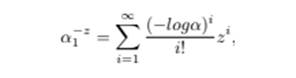
Improvement over standard distributions has gained popularity in statistical theory over the past few years. Typically, new distributions are created by combining existing distributions or adding a new parameter using generators. Alpha power transformation (APT) a novel approach for integrating an additional parameter in continuous distribution, was introduced by Mahdavi and Kundu (2017). Basically, the concept was put forth to add skewness to the baseline distribution. Then: Let g(x) be the probability density function (PDF) of a continuous random variable X.:

                                              Equation 1

 

The corresponding cumulative distribution function (CDF)

 

                                                                       Equation 2

 

Where α is the shape parameter and G(x) and g(x) are the CDF and the PDF of the baseline distribution.

Mahdavi and Kundu (2017) developed a brand-new method for creating distributions by adding a second shape parameter to a well-known baseline distribution. They used the exponential baseline distribution to introduce the alpha power exponential distribution, and they researched the fundamental characteristics as well as parameter estimation for the suggested distribution. Alpha power Weibull distribution (APWD) was introduced by Nassar et al. (2017). The capacity of APWD to simulate monotone and non-monotone failure rate functions, which are often used in reliability studies, is what gives its significance. Moments, quantiles, entropy, order statistics, mean residual life function, and stress-strength were among the attributes of APWD that were discovered. The parameters were estimated using the maximum likelihood method. The significance of the APWD was demonstrated using of actual data sets. Devi et al. (2017) introduced the entropy of the Lomax probability distribution. They derived entropy of a Lomax probability distribution as well as their order statistics which is used in business, economics, actuarial modelling, waiting problems, and biological sciences.

This study’s objective is to provide a new more adaptable distribution. The structure of this article is as follows: We go over the distribution of Alpha power Lomax (APL) in Section 2. In Section 3, new statistical properties are investigated. The Renyi entropy is derived in Section 4. In Section 5, the stress-strength reliability is described. Section 6 presents the order statistics from the Alpha power Lomax. Section 7 examines estimate techniques. Section 8 provides a simulation study. In Section 9, application is offered.

 

2. ALPHA POWER LOMAX DISTRIBUTION

In this section, we will define a new model is called alpha power Lomax distribution, denoted (APL), with three parameters (α, λ, β).

According to El-Houssainy et al. (2016) cumulative’s distribution function of Lomax distribution with scale parameter λ > 0 is

 

                                                                 Equation 3

 

where, β > 0 and λ > 0.

 

The probability density function corresponding to (3) reduces to

                                                                     Equation 4

 

The CDF of APL is generated by renaming Equation 3 as a baseline cumulative function in Equation 2.

 

                                                             Equation 5

 

and corresponding PDF of APL is defined as follows

 

                                                      Equation 6

 

where λ is the scale parameter and α is the shape parameter.

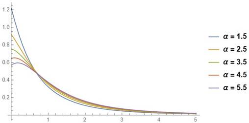
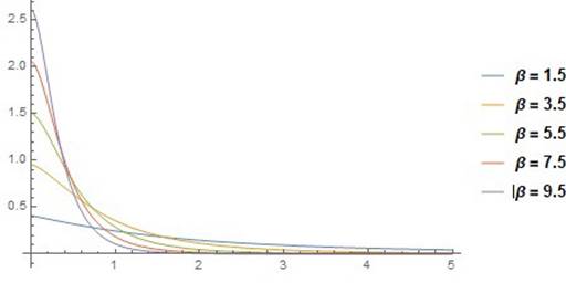
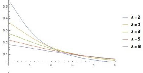
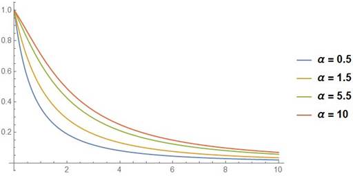
The PDF curves for the APL distribution are shown in Figure 1, Figure 2, Figure 3 with various parameter values.

Figure 1

                                                                     

Figure 1 The APL’s PDF curves with λ = 2, β = 3

 

Figure 2

Figure 2 The APL’s PDF curves with α = 3, λ = 2

Figure 3

Figure 3 The APL’s PDF curves with α = 3, β = 2

 

Figure 1, Figure 2, Figure 3 show that for various values of the parameters, the APLD density curve is uni- modal and positively skewed.

 

2.1. The survival and the hazard functions

The following forms could be used to represent the survival and hazard rate functions for the APL distribution, respectively.

 

                                                                     Equation 7

 

and

 

                                                                Equation 8

 

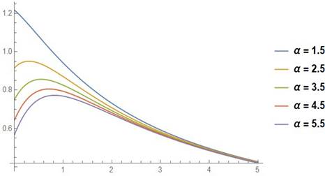
Figure 4, Figure 5 display the survival function of APLD and the hazard function for different values of parameters.

Figure 4

Figure 4 The APL’s survival function curves with λ = 2, β = 2

 

Figure 5

Figure 5 The The APL’s hazard function curves show with λ = 2 and  β = 3.

 

3. Statistical Properties

3.1. Quantile function

Let u = F (x) where U follows uniform (0, 1). By using the transformation method, we consider the random variable X of APL as follows

 

                                                 Equation 9

 

3.1.1.  THE MEDIAN

The median of the APL distribution can be obtained by putting u = 0.5 in                                               Equation 9 as follows

 

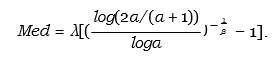                                                             Equation 10

 

3.2. The mode

The mode of the distribution can be found by solving the following equation

 

 

By taking the derivative of Equation 6 and equating it to zero and solving for x, mode becomes

 

                                                                            Equation 11

 

This is equation is not linear. The Newton-Raphson method can be used to solve it numerically.

 

3.2.1.  Skewness and kurtosis

Because the APL’s moments are not exist, we’ll apply an alternate forms using quartiles. Bowley skewness was considered as an alternate measure to determine asymmetry (Kenney and Keeping (1962)) of a distribution that takes the form

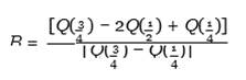
where Q represents the quantile function from Equation 9. Moors (1988) proposed a different method to determine the kurtosis of the distribution based on octiles, and it has the following form

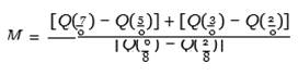
Table 1

Table 1 The Mode, Median, Skewness and Kurtosis of APL Distribution for Different Values of the Parameters.
α	λ	β	Mode	Median	Skewness	Kurtosis
4.5	0.5	2	0.000679	0.373801	0.341431	1.58388
8.5	0.5	2	0.097225	0.458852	0.327832	1.57484
12.5	0.5	2	0.148810	0.512296	0.321915	1.57231
4.5	1	2	0.001358	1.024560	0.341431	1.58388
4.5	3	2	0.004074	3.07377-	0.341431	1.58388
4.5	6	2	0.008149	6.147550	0.341431	1.58388
4.5	0.5	2.5	0.014549	0.281491	0.309599	1.50100
4.5	0.5	3	0.020491	0.225435	0.288054	1.45078
4.5	0.5	3.5	0.022919	0.187873	0.272518	1.41727

 

Table 1 the following:

1)     For constant values of λ and β, the median, mode increasing as α increases, while the kurtosis and skewness decrease.

2)     For constant values of α and β, the median and mode increase while λ is increasing but the kurtosis and skewness remain stable.

3)     For constant values of λ and α, the mode increasing as β increases, while the median, kurtosis, and skewness decrease.

 

4. Renyi Entropy of APL

Renyi entropy was invented by Renyi (1959). The variation of the uncertainty is measured by a random variable’s entropy X. Additionally, Song (2001) has effectively used the theory of entropy to a variety of applications, including information theory, engineering, and physics.

 

 

Theorem 1: The Renyi entropy of APL

                  Equation 12

 

Proof. For the density function f(x), the Renyi entropy is defined as:

 

                                                           Equation 13

 

Using  Equation 6, we obtain

 

 

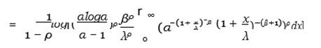
by substituting z = (1 + x) −β and using the series representation,

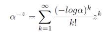                                                                          Equation 14

 

Then we have

 

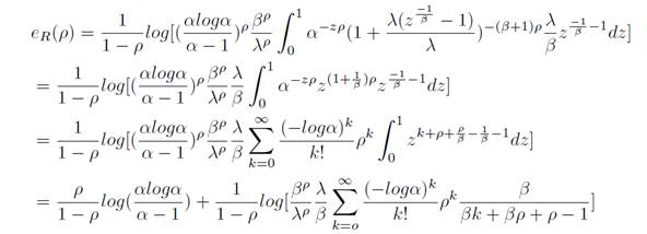
Hence, the theorem is proved.

 

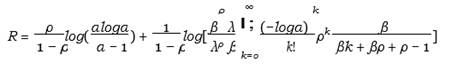
5. The Stress-Strength Reliability

In literature related to engineering, reliability, and bio statistics, the stress-strength model has attracted a lot of interest. Let X₁ represents stress and X₂ represents strength. The stress-strength model’s most basic version states that a system failure occurs when the stress exceeds the strength. Kotz and Pensky (2003). The stress-strength reliability for the APL is given by the ensuing theorem.

Theorem 5.1. The form of APL’s stress-strength reliability

 

  Equation 15

 

Proof. The stress-strength reliability can be defined as

 

 

                                                                                    Equation 16

 

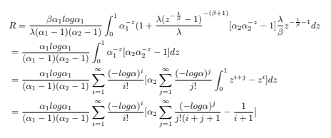
using the Equation 5 and Equation 6 of APL distribution, stress strength R, can be obtained as

 

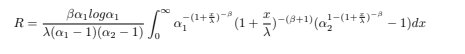
by substituting z = (1 + x) −β and using the series representation

 

                                                        Equation 17

Hence, the theorem is proved.

 

6. Order Statistics of APL

Consider  denotes the order statistic of a random sample of size n from APL distribution with CDF, F(x), and PDF, f(x), the PDF of Xr is given by Balakrishnan and Cohen (2014)

 

               Equation 18

 

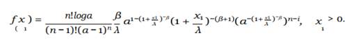
By using Equation 5,  Equation 6 the PDF the rth order statistic from APLD is given by:

 

                                                                                                                                                                                      

                                                                                                                                Equation 19

 

The PDF of the smallest order statistic, X₁, is as follows

 

    Equation 20

 

And the PDF of the largest order statistic, X_n, is given by

 

    Equation 21

 

7. METHODS OF ESTIMATION

In the section, we will study classical estimation methods to estimate unknown parameters of the APL distribution. Estimation methods that used are: (1) maximum likelihood method, (2) Ordinary least squares, (3) Weighted least squares.

 

7.1. MAXIMUM LIKELIHOOD ESTIMATION OF APL

Let X₁, X₂, ...X_n be a random sample of size n from the APL distribution. By using (6), we obtain the likelihood function L (x, α, λ, β) as

 

                                 Equation 22

 

and the log-likelihood function is

 

     Equation 23

 

     Equation 24

 

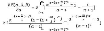
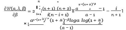
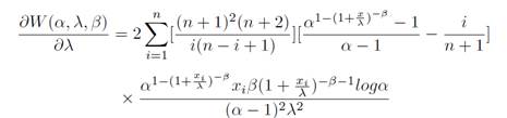
Then by deriving the log-likelihood function with respect to α, λ and β we get

 

                                             Equation 25

 

                                     Equation 26

 

                                 Equation 27

 

After solving Equation 25, Equation 26 and     Equation 27 simultaneously using the Newton-Raphson method in Mathematica 12.0, the MLE of α, β and λ could befound.

 

7.2. Ordinary Least Squares Estimation of APL

Swain et al. (1988) First suggested the least-squares estimators and weighted least-squares estimators. Assuming a random sample of size n from the APL distribution, with the observations being in the following order: x1:n < x2:n < …. < xn:n we may obtain the ordinary least squares (OLS) estimates α , λ and β as follows.

 

                                                          Equation 28

 

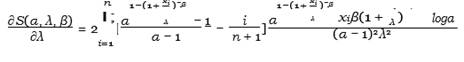
Then by deriving the S (α, λ, β) function with respect to α, λ, β, we get

 

                                        Equation 29

 

                                         Equation 30

 

              Equation 31

 

After solving Equation 29, Equation 30, and Equation 31 simultaneously using the Newton-Raphson method in Mathematica 12.0, the OLS of α, β and λ could be obtained.

 

 

 

 

7.3. Weighted Last Squares Estimation of APL

Weighted least squares (WLS) estimates are represented using the following α, β and λ form

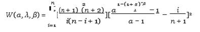                                 Equation 32

 

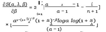
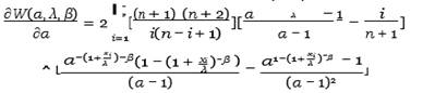
Then by deriving the W (α, λ, β) function with respect to α, λ, β, we get

 

                                  Equation 33

 

                         Equation 34

 

             Equation 35

 

After solving Equation 33, Equation 34 and Equation 35 simultaneously using the Newton-Raphson method in Mathematica 12.0, the WLS of, and could be obtained.

 

8. SIMULATION STUDY

To make sense of the theoretical findings, simulation using Mathematica 12.0 have been carried out, of the estimating issue presented in the earlier parts. Simulated research has been carried out for mean square error (MSE) and average MLEs.

The estimator computation algorithm is

Step 1: Create a random sample of size n using Equation (9) for the starting parameter values (α, β, λ).

Step 2: Use the Newton-Raphson method to solve the equations in to estimate the MLE, LSE and

WLSE of the parameter α to solve the equations given in (25), (29) and (33), respectively.

Step 3: Compute the estimator of entropy from (12), using the estimates in the previous step.

Step 4: 1000 times, repeat the first three steps.

Step 5: Calculate the MSE.

Different sample sizes of the ML estimate for α, entropy and MSE for the real parameter values are shown in Table 2. The LSE estimations for α, entropy and MSE for true parameter values are presented in Table 3. Additionally, the WLSE estimates for α, entropy, and MSE for the genuine parameter val- ues are shown in Table 4

Table 2

Table 2 The MLE and MSE for the Parameters α.
Parameters	n	Mean (α)	MSE (α)	MLE Entropy	MSE Entropy
α = 2	30	2.10996	0.055305	0.794999	0.001414
β = 4	50	2.10507	0.050296	0.794381	0.001292
λ = 3	200	2.09217	0.049327	0.792177	0.001273
ρ = 2	500	2.07664	0.041060	0.789856	0.001079
	1000	2.04933	0.031904	0.785526	0.000860
α = 3.5	30	3.49168	0.081989	0.901258	0.000717
β = 3	50	3.47555	0.080602	0.899818	0.000716
λ = 2	200	3.47064	0.078377	0.899322	0.000695
ρ = 2	500	3.47054	0.074389	0.893239	0.000648
	1000	3.44995	0.065321	0.893229	0.000566
α = 5.5	30	5.49820	0.084452	1.815170	0.000363
β = 3	50	5.49050	0.083072	1.814670	0.000359
λ = 2	200	5.48660	0.082376	1.814400	0.000352
ρ = 2	500	5.47801	0.079926	1.813870	0.000345
	1000	5.47643	0.075352	1.813790	0.000326

 

Table 3

Table 3 The LSE and MSE for the parameters α.
Parameters	n	Mean (α)	MSE (α)	MLE Entropy	MSE Entropy
α = 2	30	2.167800	0.059513	0.804842	0.001468
β = 4	50	2.166970	0.057549	0.804195	0.001427
λ = 3	200	2.133420	0.045056	0.799589	0.001126
ρ = 2	500	2.087780	0.029733	0.792361	0.000760
	1000	2.008250	0.010686	0.779427	0.000294
α = 3.5	30	3.464680	0.087933	0.898712	0.000789
β = 3	50	3.453120	0.083220	0.897577	0.000744
λ = 2	200	3.385090	0.082102	0.891249	0.000713
ρ = 2	500	3.277550	0.079814	0.881001	0.000697
	1000	3.171800	0.051935	0.870616	0.000321
α = 5.5	30	5.482420	0.084139	0.885941	0.000360
β = 2	50	5.457720	0.083646	0.884451	0.000351
λ = 1	200	5.412630	0.083646	0.881737	0.000321
ρ = 2	500	5.307800	0.073992	0.874050	0.000316
	1000	5.192590	0.073594	0.868265	0.000207

 

Table 4

Table 4 The WLSE and MSE for the Parameters α
Parameters	n	Mean (α)	MSE (α)	MLE Entropy	MSE Entropy
α = 2	30	2.176210	0.062294	0.806236	0.001535
β = 4	50	2.172040	0.060366	0.805593	0.001495
λ = 3	200	2.171150	0.059024	0.805502	0.001487
ρ = 2	500	2.167290	0.059968	0.804785	0.001462
	1000	2.164850	0.056621	0.804519	0.001402
α = 3.5	30	3.476270	0.089437	0.899785	0.000800
β = 3	50	3.463550	0.087462	0.898549	0.000778
λ = 2	200	3.46067	0.084138	0.898370	0.000747
ρ = 2	500	3.453780	0.083912	0.897605	0.000754
	1000	3.451360	0.082047	0.897472	0.000734
α = 5.5	30	5.483850	0.086180	0.886005	0.000312
β = 2	50	5.483810	0.085978	0,886004	0.000311
λ = 1	200	5.480090	0.084704	0.885813	0.000308
ρ = 2	500	5.474100	0.082359	0.885431	0.000301
	1000	5.458950	0.081502	0.884541	0.000295

 

From Table 2, Table 3, Table 4, we observed that the MSE of the estimate α and entropy decreases as the sample size increase. Also, the mean of the estimate α and the MLE of entropy decreases as the sample size increase.

 

9. Applications

In this section. The inverse Lomax distribution (ILD) introduced by Hassan and Mohamed (2019) and the exponential lomax distribution (ELD) introduced by Abdo et al. (2015) will be used to compare the fit of the APLD with other lifetime models that are well-known. Additionally, we take into account the model selection parameters, such as the Akaike information criterion (AIC), log-likelihood (), Bayesian information criterion (BIC), consistent Akaike information criterion (CAIC), and Hannan-Quinn information criterion (HQIC). The lowest values of AIC, BIC, CAIC, HQIC and greatest value of,  all point to a better fit of the data, Where

 

 

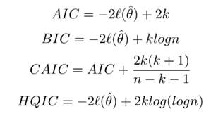
k is the number of parameters; n is the sample size and (θˆ) is the log-likelihood function evaluated at the highest likelihood estimates.

Data I: COVID-19 cases every day in Saudi Arabia

From 1 April to 2 May, this information reveals the daily COVID-19 instances in Saudi Arabia. These statistics were obtained from the Saudi Ministry of Health’s website, located at https://covid19.moh.gov.sa.  These findings are

110, 157, 165, 154, 140, 206, 138, 272, 137, 355, 364, 382, 429, 472,435, 493, 518, 762, 1132, 1088, 1122,

1147, 1141, 1158, 1172, 1197,1223, 1289, 1266, 1325, 1351, 1344, 1362.

Table 5 displays descriptive statistics for this data.

Table 5

Table 5 Descriptive Statistics for the Number of Daily COVID-19 Cases in Saudi Arabia
Measure	Value	Measure	Value
N	33	Minimum	110
Maximum	1362	Mean	727.455
Q1	255.5	Q3	1178.25
Median	518.	Skewness	0.0350687
Kurtosis	1.26721	Variance	230684.0
Standard deviation	480.295

 

The performance of the APLD in comparison to other models is shown in Table 6 along with the MLEs for the model parameters.

Table 6

Table 6 MLEs of the Model Parameters and the Statistics of the AIC, BIC, CAIC, HQIC and for the Number of Daily COVID-19 Cases in Saudi Arabia
Distributions	MLE α	MLE entropy		AIC	BIC	CAIC	HQIC
APLD	34.7454	2.73066	-243.261	492.532	497.012	493.350	494.033
ELD	0.04329	0.39915	-425.628	857.257	861.746	858.085	858.768
ILD	182.650	2.95628	-253.035	512.070	516.560	512.898	513.581

 

Table 6 shows that, among the models taken into consideration, the APLD has the smallest AIC, CAIC, BIC, and HQIC values. Which shows that the APLD seems to be a model that might work well with the data set.

Data II: (Natural phenomena) Badr (2019) presented the consist of 30 successive March precipitation (in inches) observations.

77, 52, 90, 174, 162, 205, 81, 131, 120, 32, 195, 95, 120, 81, 47,281, 143, 187, 337, 118, 220, 135, 300,

475, 309, 248, 151, 96, 210,189.

Table 7 displays descriptive statistics for this data.

Table 7

Table 7 Descriptive Statistics for the of 30 Successive March Precipitation (in inches)
Measure	Value	Measure	Value
N	30	Minimum	32
Maximum	475	Mean	168.7
Q1	95.	Q3	210.
Median	147.	Skewness	1.12002
Kurtosis	4.30607	Variance	9786.15
Standard deviation	98.925

 

The performance of the APLD in comparison to other models is shown in Table 8 along with the MLEs for the model parameters.

Table 8

Table 8 MLEs of the Model Parameters and the Statistics of the AIC, BIC, CAIC, HQIC and for the of 30 Successive March Precipitation (In Inches)
Distributions	MLE α	MLE entropy	,e	AIC	BIC	CAIC	HQIC
APLD	66.161	2.83245	-200.811	401.622	412.201	408.422	409.183
ELD	0.0370132	0.351725	-476.589	959.178	963.757	959.978	960.739
ILD	440.78	3.040180	-296.266	598.532	603.111	599.322	600.093

 

Table 8 is results show that while, e has the largest value and the APLD has the smallest AIC, CAIC, BIC, and HQIC values. As a result, the APLD performs better than other models.

 

CONFLICT OF INTERESTS

None. 

 

ACKNOWLEDGMENTS

None.

 

REFERENCES

Abdo, N. F., El-bassiouny, A. H. and Shahen, H. S. (2015). Exponential Lomax Distribution. International Journal of Computer Applications, 121, 14-29. https://doi.org/10.5120/21602-4713.

Badr, M. M. (2019). Goodness of Fit Tests for the Compound Rayleigh Distribution with Application to Real Data. Heliyon, 5,1-6. https://doi.org/10.1016/j.heliyon.2019.e02225.

Balakrishnan, N. and Cohen, A. C. (2014). Order Statistics and Inference: Estimation Methods, Academic Press, San Diego, California.

Devi, B., Kumar, P. and Kour, K. (2017). Entropy of Lomax Probability Distribution And Its Order Statistic. International Journal of Statistics and Systems, 12(2), 175-181.

Dey, S., Nassar, M. and Kumar, D. (2019). Alpha Power Transformed Inverse Lindley Distribution : A Distribution With an Upside-Down Bathtub-Shaped Hazard Function. Journal of Computational and Applied Mathematics, 130-145. https://doi.org/10.1016/j.cam.2018.03.037.

El-Houssainy, A., Rady, W. and Elhaddad, T. (2016). The Power Lomax Distribution With an Application to Bladder Cancer Data. Springerplus, 1838,1-22. https://doi.org/10.1186/s40064-016-3464-y.

Hassan, A., and Mohamed, R. (2019). Weibull Inverse Lomax Distribution. Pakistan Journal of Statistical and Operation Research, 587-603. https://doi.org/10.18187/pjsor.v15i3.2378.

Ijaz, M., Asim, S. M. And Alamgir, M. (2019). Lomax Exponential Distribution With an Application to Real-Life Data. Plos One, 12-14. https://doi.org/10.1371/journal.pone.0225827.

Ihtisham, S., Khalil, A., Manzoor, S., Khan, S. A. and Ali, A. (2019). Alpha-Power Pareto Dis- Tribution its Properties and Applications. Plos One, 6-14. https://doi.org/10.1371/journal.pone.0218027.

Lomax, K, S. (1954). Business Failures: Another Example of the Analysis of Failure Data. Joumal of the American Statistical Association, 49, 847-852. https://doi.org/10.1080/01621459.1954.10501239.

Kriver, J. F. and Keeping, E. S. (1962). Mathematics of Statistics, 3rd edition, Part 1, Princeton, New Jersey.

Kotz, S. and Pensky, M. (2003). The Stress-Strength Model and its Generalizations : Theory and Applications, World Scientific, New Jersey. https://doi.org/10.1142/9789812564511.

Mahdavi, A. and Kundu, D. (2017). A New Method for Generating Distributions with an Application to Exponential Distribution. Communications in Statistics- Theory and Methods, 46(13), 6543-6557. https://doi.org/10.1080/03610926.2015.1130839.

Moors, J. (1988). A Quantile Alternative For Kurtosis, Journal of the Royal Statistical Society : Series D (The Statistician), 37, 25-32. https://doi.org/10.2307/2348376.

Nassar, M. Alzaatreh, A., Mead, M. and Abo-Kasem, O. (2017). Alpha Power Weibull Distribution : Properties and Applications. Communications in Statistics Theory and Methods, 20(46), 10236-10252. https://doi.org/10.1080/03610926.2016.1231816.

R'enyi, A. (1959). On The Dimension and Entropy of Probability Distributions. Acta Math. Hung. 10, 193-215. https://doi.org/10.1007/BF02063299.

Song, K.S. (2001). R'enyi Information, Loglikelihood and an Intrinsic Distribution Measure. J.Stat. Plan. Inference 93, 51-69. https://doi.org/10.1016/S0378-3758%2800%2900169-5.

Swain, J., Venkatraman, S. and Wilson, J. (1988). Least Squares Estimation of Distribution Function in Johnson's Translation System. Journal of Statistical Computation and Simulation, 29, 271-297. https://doi.org/10.1080/00949658808811068.