Random waypoint mobility routing Algorithm for Mobile Sensor Networks

 

S. Hemalatha ¹, Dr. E. George Dharma Prakash Raj ²

 

¹ Programmer, IT Support, Bishop Heber College, Trichirapalli, Tamil Nadu, India

² Associate Professor, School of Computer Science, Engineering and Applications Bharathidasan University, Tiruchirappalli, Tamil Nadu, India

 

1. INTRODUCTION

Mobile sensor dynamically self-configure and self – organized network. Self-configured network to identify the neighbouring node is highly challenging. The cluster of movable sensors grouped to form a cluster region. Periodically routing table is updated because Sensor nodes are capable of changing their locations from time to time. In general, mobility can be applied neither nor to all the nodes.

A node can be either active or passive. In the case of Active nodes, capable of changing its locations based on the real-time scenario. On the other hand, while in passive nodes, changing its locations assisted by human or environmental conditions.

The Mobile sensor networks (MSN) are widely used for monitoring larger application's health care, environmental monitoring, to border security on the nation, and real-time industrial sectors, habitat monitoring, traffic observing, battlefield surveillance, rescue operations, smart homes, smart cities, and flexible extensions of mobile sensor networks.

Less mobile or dynamic low-energy sensor nodes make up mobile sensor networks. These sensors work together to create a self-contained distributed network. The information about perceived objects inside the network coverage area is collectively perceived, collected, processed, and transmitted via a distributed network and wireless communication medium. Initially, sensor nodes were randomly dispersed.

Sensor node is tiny ones has Contains a limited battery life. Periodically the routing table is updated because sensor nodes are keep changing its location due to mobility factor, it leads to an additional computational complexity added to routing.

Mobile sensor network can be further classified into 2 different types there are,

1)     The Inter cluster based, and

2)     The Intra cluster-based network.

 

In Inter cluster-based network, Sensor Nodes are connected directly / indirectly to the cluster head without any hierarchical order. In Intra cluster based Mobile sensor network follows different topological structure, scalable mechanisms, and routing function. Geographical location of the individual sensor and its neighbours obtained by Localization algorithm (Global Positioning System).

Mobile sensor network build by a Mesh topological structure, Multi cast routing protocols used to improve packet delivery ratio, and network lifetime. Mesh topology reduces installation overhead, distribution of workloads and maintenance cost. Using mobile network resources like the global system for mobile communication (GSM), general packet radio service (GPRS), and code division multiple access, which are built and maintained by telecom operators, long-distance wireless communication can ensure the real-time and dependability of data transmission. Nodes in a mobile sensor network don’t rely on any pre-existing infrastructure. Instead, the nodes themselves form the network and communicate within radio frequency range.

Sensor Nodes mobility factor frequently will change   topology structure and path break occurs during the data transmission. To swiftly react to topological changes and effectively find an alternate way, routing protocols should be designed. On the other hand, the Mobile Sensor Network has significant difficulties due to the restricted power and bandwidth resources in mobile nodes.

 

2. LITERATURE SURVEY

The most well-known hierarchical routing protocols created for sink-based Mobile Sensor Networks are covered in this section, and Table 1 discusses their features.

Wireless sensor networks that use software to define them (SDWSNs). In order to choose the optimum routing protocols to be deployed over various time frames in line with application-specific criteria, we use the supervised learning approach in decision-making.

The Software Defined Network controller adapts, introduces the selected protocol into the network. While modifying the application's specific requirements. In terms of consumption of residual energy, Packet delivery rate and network packet delivery delay, the suggested solution performs better than the ones currently in use. Existing methods employ a particular protocol for various time frames.

Partial-Partitioned Greedy Algorithm for Routing proposed to inter and intra cluster based mobile sensor network. Author proposed three heads, such as Cluster Head, First Transmission Head and subordinate Transmission Head for each cluster, in    this selection made up of the node's remaining energy inside the cluster. Highest residual energy node elected as CH and next higher energy node is elected as     FTH, and the next prior energy node get elected as the STH, STH->FTH->CH.

Cluster head communicate the base station during the data request and transmission. Each time interval t seconds, the routing table is get updated and the corresponding CH, FTH, STH get selected in the cluster Hemalatha and Prakash Raj (2019). The packet loss and EED are reduced as a result of load balancing of the heads. Conversely, it causes the network's energy usage and delivery ratio to decline. A load-balanced routing strategy has been devised for mobile sensor networks; the highest residual energy node is chosen as the cluster leader. Sensor nodes automatically migrate in and out of the cluster region from time to time. If CH left the cluster, the new CH would be chosen by projecting its future location, which a sensor node would then broadcast to any other nodes that were within range. Otherwise, the new cluster head in LBRP Chatterjee et al. (2017) is chosen at random from a sensor node near to the current CH.

According to the node's speed and density, mobile sensor networks force nodes to be mobile and inherit the behaviour of the network Alagu Pushpa et al. (2011).

Table 1

Table 1 Overview of Hierarchical Routing Table
Algorithm for Routing	Mobility  Pattern of Sink  node	Virtual topological  structure	Dissemination	Strategy for  routing data on MSN	End to End Delay	Residual Energy consumed
CCM-GR	Static/ Random	Unit Disk Graph	Sink location	Greedy	Low	High
EPFA	Random	Cluster region	Sink location/ Data transfer	Greedy	Medium	High
PPGA	Random	Intra cluster	Route discovery/ data transfer	Cluster b8ased	High	Medium
RWMRA	Random	Intra cluster	Route discovery/ data transfer	Random waypoint model	High	Medium

 

According to the proposed work setup with the Ad hoc on Distance Vector and DSDV routing protocols, the network's performance is determined by the node density, hop count, pocket loss ratio, and node velocity. Compared to DSDV, AODV increases packet delivery ratio and reduces pocket loss. The node's mobility, including its direction, speed, and remaining energy, is the main focus of the DDR protocol. a pie-shaped area that is utilized to connect with the base station and is defined by an angle of 60 degrees with regard to the base station's position Almesaeed and Jedidi (2021).

 Within the communication range r, find the Euclidean distance neighbor towards sink in the cluster region towards    the base station. DDR enhances the packet delivery rate and energy. Socratic Random Algorithm (SRA) Murugan and Khan Pathan (2019) fortify an efficient target coverage and network connectivity of mobile Sensor Network to extend the life time of sensor nodes Murugan and Khan Pathan (2019).

In order to save energy and improve data dependability for mobile sensor networks, a round time estimation scheme is developed. The time period after which the role of a sensor node should change from CH to non-CH and vice versa must be determined in order to preserve energy and increase data transfer to the destination. An improved perimeter forwarding technique for a sensor network based on inter-cluster clusters is proposed. EPFA Hemalatha and Prakash Raj et al. (2019) the node is clustered as a single cluster in which all highest residual energy node is get selected as a cluster head, all the other nodes treated as cluster members. In some cases, in use greedy forwarding, few cases uses perimeter forwarding based on the neighbouring node, routing table is periodically get updated in each rounds. Reliable Energy Aware Routing Protocol (RER), which calculates the distance between the current node and the relay node, the relay node's distance from the sink node and the current node's remaining energy, and the link quality. Reliable Energy Cost Based on Distance (RECBD) is used to route messages Ma et al. (2019).

RECBD to improve sensor network reliability, delivery ratio, reduce energy consumption and prolong the network lifetime. Situation aware protocol is proposed for Inter cluster and Intra cluster-based routing taken for the major aspect in this paper Hemalatha and Prakash Raj (2020). In mobile sensor network are widely fall in intra cluster-based network until some specified applications are not requires the intra cluster-based routing. Find directions and nearest neighbour play a vital role for routing. Energy of the sensor node is restricted over a limited time, and mobility of the node is unpredicted, so packet routing needs a new routing algorithm to be dynamic sensor network.

Energy-efficient Nonlinear Coverage Control Protocol (ENCP) proposed for mobile sensor network Sun et al. (2018). Scheduling of all nodes in done by collaboratively. Energy Nonlinear Coverage protocol applied with minimum number of sensors. So, the coverage of the network is gained. So, energy consumption is confirmed. Model of a dynamic cell routing network. In order to create a sensing distance inside a radius communication system between various sensors. When the nodes are moving, this protocol observes cell formation and re-construction. The main feature of this algorithm Yang et al. (2009) is to introduce localization of the cell reconstruction in order to calculate the routing paths without modifying unnecessary cells throughout the entire network.

The RWMRA's region maintenance technique eliminates hotspot issues. In the section that follows, the proposed RWMRA is studied in detail. The remaining text is divided into the following sections: The proposed random waypoint routing algorithm for mobile sensor networks is presented in Section 3, the problem statement and system definition are defined in Section 2, the results and discussions are discussed in Section 4, and the conclusion is presented in Section 5.

 

3.    SYSTEM MODEL / PROBLEM STATEMENT

   Network is segmented by D * D regions, Mobile sensors randomly deployed, S={s1, s2,  s3 .., 𝑠𝑛} initially located in a random location, time interval various from T = {t1, t2, t3,t4,      , tm} mobility

   assumed by speed 10,15,20,25 and 30, Interval 0.2 to 2.2, Pause Interval 0 to 1, Direction Interval - 180, 180 assigned to the nodes.

The system function model is defined as follows:

1)     Choosing Region head by perceive the low energy and denying them from RH nomination.

2)     To ensure connectivity and target coverage in a dynamic network. Our main concern is figuring out which way and where the sensors should travel. For the given time interval. To exchange information between coverage sensor nodes and the sink, sensor nodes should move in a straight line to reach the target's coverage area.

3)     Based on the goal route's velocity and acceleration, sensor nodes are separated into regions, each of which is allocated a region head. The remaining nodes are each given an area id.

4)     Model of mobility. Sensor nodes are unrestrictedly free to move in and out of the given zone in any direction. The network's nodes move according to an application's requirements, and the node's velocity is determined there.

 

V=

dx-speed in X-Axis,

dy-speed in Y-Axis.

 

The Acceleration of the node is calculated by,

 

Acceleration =

 

The Energy consumption calculated by,       

 

EC =

 

Data transmission between coverage sensor nodes and the sink is required during the specified time period, sensor nodes must move in a straight line through the region to the target's coverage area.

 

4. RANDOM WAYPOINT MOBILITY ROUTING ALGORITHM

The RWMRA applied on virtual infrastructure based mobile sensor network. Sensor nodes lying on the virtual regions are called virtual sensor nodes (VS nodes). Each routing table maintained to store current location, and update location for the regular time interval T seconds. RWMRA algorithm proposed to find the neighbourhood node, the reliable path towards sink location and transmit data.

 Due to their handling of the majority of network traffic, VS nodes experience faster energy depletion. RWMRA therefore includes a pause time mechanism. The deployment of nodes is illustrated step-by-step in Algorithm 1.

The following are the presumptions that were taken into account when designing and developing RWMRA.

1)     A range of N homogenous SN’s are randomly arranged in a 2D sensor field with flat surfaces.

2)     The radio range of each sensor node is fixed. Sink uses a notion of mobility with random waypoints.

3)     Each sensor node Si is aware of the location of the deployment region's centre point C (xc; yc) as well as its own location Si (x; y).

4)     Due to mobility the nodes moves in and out around the region.

5)     Time interval T seconds, repartitioning is established to proceed the steps to configure the sink node.

 

4.1. REGION CREATION

There are three important aspects to construct a virtual region:

1)     Sensor region partitioning.

2)     Calculate the Distance from current node Against Virtual Sink node.

3)     Path selection and joining of VS node

 

4.1.1.  Sensor region partition

 

Phases of Figure 1. Here, summarizing the region's construction phase

Figure 1

                                                                     

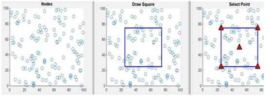
Figure 1 Region creation a). Node deployment b). Region creation D*D c).  Region head

 

Algorithm 1: Region Creation

1)     Randomly deploy sensor nodes.

2)     Partition the sensor field into D regions.

3)     Select center point and corner points

4)     Create region head (SSN) based on selected region

5)     Draw circle based on the selected points using.       .   radius 𝑟_{𝑐𝑜𝑚𝑚}

6)     For each node in Network

7)     Get node location n(x,y)

8)     For each region in Network

9)     Get the location of ssn(x,y)

10) Compute the dist(x,y) = n(x,y) - ssn(x,y)

11) If (dist (x,y) ≤ 𝑟𝑐𝑜𝑚𝑚)

12) Set node n coverage = Yes

13) break.

14) Else Set node n coverage = No

15) EndIf

16) EndFor

17) EndFor

 

4.1.2. PARTITIONING OF SENSOR FIELD

The sensor field is divided by RWMRA into a D equi- distance zone. Each area has a region head with the following radius values: r1, r2, r3,..., rk. The partitioning of the sensor field is shown in Figure 1. Equation allows for the determination of the ideal number of areas (1),

 

𝑁𝑢𝑚𝑏𝑒𝑟 𝑜𝑓 𝑅𝑒𝑔𝑖𝑜𝑛𝑠 =

 

{         𝑋,                𝑖𝑓 𝑌 ≤ 𝑟𝑐𝑜𝑚𝑚} ------------ (1)

                                         𝑋 + 1,    otherwise

[

                                       Where X=   y=

                                          Radius’s of the nth Region is 

Where r=1<n≤k

 

Figure 2

                                                                     

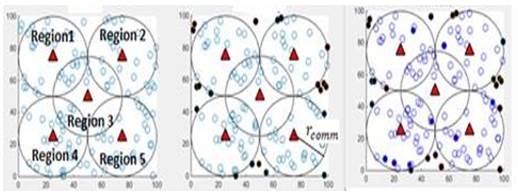
Figure 2 Advertise Mobile sink location a). node inside of all the region b). node outside of all the region c). node in between the region

 

4.1.2.  SELECTION OF CURRENT NODE \ VS SINK NODE

Nodes are chosen as the current node VS neighbourhood node depending on their distance from the nearest region after the number of regions has been established and their radii have been determined. Sink broadcasts Region info MSG [(r1, r2, r3,..... rk), (R1, R2, R3.........Rk)] at the start of phase, comprising the radius of each region and its corresponding region no (i.e., n = 1,2,3….k). A sensor node I recognizes itself as a VS current node belonging to the nth area upon obtaining this information If the distance between it and the network is Euclidean (n), center falls within the range.

𝑟   − ∞ < 𝐷𝑛 < 𝑟− ∞, nodes to the sink.

                                                                                             

Where ∞ < 𝑅_{𝑐𝑜𝑚𝑚} /2 (see Figure 2b).

 

5. PATH SELECTION AND JOINING VS NODE

During this stage, a portion of the candidate VS nodes join together to form the region and develop into VS nodes. The VS nodes are in charge of keeping track of the sink's position information and data transmission from the source node to the sink. As seen in Figure 2c, region is a one-node-width virtual structure that encloses the network core. A simple and energy-efficient system, region construction works from the region head to the region MEMBERS.

 

6. NEIGHBOURHOOD DISCOVERY

All of the regular sensor nodes locate the closest VS node during this phase, which enables them to transmission of data to the sink. Sink node broadcast Nbrinfo MS [Ri,ID, Si (x, y)] containing their respective region number, ID, and location during the neighbour discovery process. Normal sensor nodes that get Nbrinfo MSG from various VS nodes figure out their distances from them, and for a given sensor node, the VS node with the smallest distance is chosen as its neighbour. Each sensor node also indicates whether it is inside or outside the zone based on its position in relation to it.

 

7. MOBILE SINK LOCATION ADVERTISEMENT

The primary function of VS nodes is to communicate source node data to the mobile sink, and in order to do so properly, they need to be aware of the sink's most recent location. As a result, when a mobile sink spends time in a single area, it updates the VS nodes with its location as per Algorithm 2. In order to do this, the sink transmits a Sinkinfo MSG Sink(x, y), stop time I containing its position and pause time, either in the angle of the network Centre if it is outside of all rings or away from the network centre if it is inside all regions (See Figure 2a) (See Figure 2b). The mobile sink, on the other hand, delivers Sinkinfo _MSG in both directions if it is between two regions (See Figure 2c).

The initial VS node that receives a Sinkinfo MSG records the sink's most recent location and passes it along to both its clockwise and counterclockwise neighbouring VS nodes and other rings. Only after a VS node receives Sinkinfo MSG from both of its clockwise and anticlockwise neighbouring VS nodes does this procedure come to an end. In this manner, the most recent location of the sink is made known to all VS nodes. The following section explains how VS nodes use this knowledge to transmit information from source nodes to sink nodes.

 

ALGORITHM 2: ANNOUNCE MOBILE SINK LOCATION

1)     if distance (dest (x, y), C (xc, yc)) ≤ r1 then

2)     send a destinfo_MSG in the opposite direction of the network center

3)     else if distance (dest (x, y), C (xc, yc)) ≥ rk then

4)     send a destinfo_MSG towards the network center 5 else

5)     send two destinfo_MSG; one towards the network center and one in the opposite direction of the network center.

6)     for each node receiving destinfo_MSG do 8 if Node i : type == normal sensor node then 9 Ignore the destinfo_MSG

7)     else

8)     if (Previous destination location! = Current destination location) then

9)     Save the destination location information, share destinfo_MSG with its clockwise and anti- clockwise neighbouring VS nodes, and other region.

10) stop sharing destinfo_MSG 14 else

11) send the destinfo_MSG to its next neighbouring VS node

12) Ignore the destinfo_MSG

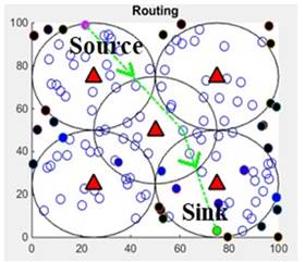
Figure 3

                                                                           

Figure 3 Data Transmission Source node Sink node

 

7.4. DATA TRANSMISSION

Figure 3 shows the process for multi-hop data communication from the source node to the mobile sink. It is based on Algorithm 4. The S_Node delivers Data MSG Data to its neighbouring VS node since VS nodes serve as data forwarders and contain the updated position of the sink. When the Data MSG is received, the VS node uses an angle-based routing technique to transfer this packet to one of its two anticlockwise) directions, which is the mobile sink.

It aids in selecting the following suitable VS node with the goal of transmitting data to the sink with the shortest possible path. This process states that the VS node selects the neighbouring VS node that has the smallest angle with the sink. The information is continued to be routed to other VS nodes until it arrives at a VS node that is only one hop away from the sink.

After announcing the path, the system checks logically to see if the previous sink location and the current sink location are the same. If they are not, the packet is forwarded along the same route while waiting for the node's status (NS=wait, Noncoverage/coverage), according to Workflow Diagram 1. This will lower the ratio of packet losses.

Sends Data MSG to the closest VS node R1 in Figure 3. R1 can transfer the Data MSG to the gateway through two nearby nodes (R1 and R5). Since R3CSN is closer to R2CSN than either of these two neighbouring nodes, R1 chooses R3 by employing an angle-based routing strategy. Additionally, R3 passes this Data MSG on to its subsequent neighbouring VS node, and so on, until the message reaches the sink. Each VS node receiving Data MSG from any source node follows the same process. A VS node aggregates the data before sending it to the sink if it gets Data MSG from two or more source nodes or its neighbouring VS nodes. Depending on the user's requirements, VS nodes here conduct basic data aggregation operations on the sensed data received from source nodes, such as max, min, average, etc.

 

ALGORITHM 3: DATA TRANSMISSION

1)     compute the distance between X and Y at interval time t

2)       dis^X,Y(t) =|| Xloc(t) – Yloc(t) || 2: if dis X,Y(t) ≤ 𝑟𝑐𝑜𝑚𝑚

(Node X is within the transmission range of

3)     Node Y) then

4)     NS = Get node status ()

5)     If (NS == Coverage)

6)     Transmit Data

7)  Else If (NS == Non Coverage)

8)     Exit routing

9)     Else If (NS ==Move)

10) Wait until Node movement

11) Else (Node X is not in the transmission range of Node Y)

// Use Node Y nearest SSN to Compute 11:    D1= || SSNloc (t) – Yloc (t) ||

12) `D2 = || SSNloc (t) – Yloc (t+1) ||

13) DC = ||D2 – D1|| / D1

14) θ = || θ (t+1) – θ|| / 2π

15) mob = α. DC + β. θ (Where α and β ϵ [0, 1])

16) Find the path based on mob

17)  Check all nodes (path) mobility status

18) Update the pause time of node

19) Transmit data

Figure 4

                                                                     

Figure 4 Data Transmission

 

A Single hop data transmission from source to destination shown in Figure 4. In the occurrence region5 the source node transmit the data to region 2, using the algorithm 2. Ultimately improves Packet delivery ratio, Energy on the network. RWMRA is performs better than PPGA.

 

8. SIMULATION AND PERFORMANCE

We performed simulations on Mat lab for the performance          comparison and evaluation of  RWMRA with PPGA and EPFA. In our simulation, we consider a space of 200m X 200m in which 120 nodes are deployed randomly to form a network. Nodes deployed at random order. Here each packet begins its trip from a random manner. On the basis of the chosen characteristics, such as the PDR, EED delay, node collision, and energy consumption, the suggested Random waypoint mobility routing is evaluated. RWMRAA performed better than PPGA and EPFA in terms of chosen cluster heads per round and packets to BS.

The implemented in matlab, results shows the proposed technique achieves packet delivery ratio and energy conservation in order to improve network lifetime. Every time, the mobile node selects a random destination and moves there at a uniformly distributed speed between [v0, max], where Vmax is the highest speed that a node is permitted to travel at.

Once there, the node stops for the amount of time specified by the "time to live" option. Once this time has passed, it again selects a random location and repeats the entire process until the simulation is over.

Table 2

Table 2 Simulation Setup
Parameters	Values
Network area (M × M)	200 × 200 m2
Number of sensor nodes (N)	120 nodes
Node density (nodes per square meter)	0.003
Initial energy of deployed node	30 Jules
Transmission range, r (meters)	20 meters
Time Interval	20 seconds
Maximum node velocity(meters per sec)	5, 10, 15, 20, 25
Packet size (bytes)	32 bits for AODV 64 bits for OLSR
Speed Interval	0.2 to 2.2 seconds
Direction Interval	-180, 180 Degree
Simulation interval	2000 rounds

 

9. METRICS

In order to compare the performance of the various routing protocols, we have chosen the packet delivery ratio, average EE_D delay, packet collision, and energy consumption metrics during the simulation.

 

9.1. PDR PACKET DELIVERY RATIO

PDR is a difference between total numbers of packets successfully received by the destination node, the number of packets sent by the source node for the time interval T.

 

PDR=           ∗ 𝑇𝑖𝑚𝑒

 

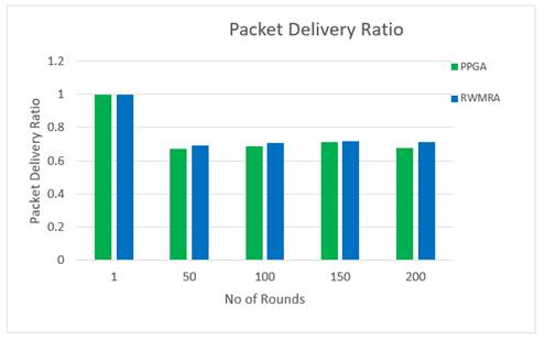
Figure 5

                                                               

Figure 5 Packet Delivery Ratio

 

Figure 5 express packet delivery ratio with respect to time interval T rounds with approximately 120 sensor nodes. The result shows that the packet delivery ratio of the RWMRA algorithm various from time interval t. From Figure 4.1 RWMRA recovers highest delivery ratio among PPGA. EPFA provides the best connectivity compared with non- position based sensor network.

From the results, it can be inferred that region-based routing systems require a recovery strategy because it helps to increase the packet delivery ratio while moving. We can determine how effectively the protocol delivers packets to the application layer using this estimate. A high PDR number is a reliable sign of a protocol's effectiveness because it shows that the majority of packets are reaching the higher tiers. When a subscription succeeds, that.

Sending a subscription message to the network and receiving corresponding awareness data both require a subscriber. In general, the algorithm takes longer to process the more published event content there is to be analysed. As a result, event transmission to subscribers takes longer, which reduces the processing speed of events. The average amount of time needed for subscribers to correctly receive published events is compared in Simulation 1. Three publish/subscribe messaging methods with various published event counts were used to run the experiment.

 

9.2. EED END-TO-END DELAY

This is derived using the formula below and is known as the typical packet transmission delay between two nodes.

EED = -

i------Packet identifier

---Reception time of packet i

---Sending time of packet i

n-----Number of packets successfully delivered

Figure 6

                                                                     

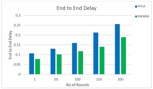
Figure 6 End to End Delay on Nodes

 

Figure 6 shows the end to end delay in each time interval round. In random way point model are responsible to obtain the region head, to find the next hop towards the destination on regular time interval for 2 to 3 seconds. Data packets from sensor node, find the optimal path from single / multiple hop to determine shortest routing path to reach the destination.

It is the responsibility of the region heads to gather the sensed data from the sensor nodes, then to transfer it to the BS. Following the conclusion of every round, new Region heads are selected. To maintain a balance in the energy consumption of the sensor nodes, the Region head is chosen at random. A minimum number of RHs will need them to gather, transmit, and receive data from more sensor nodes, which will use up more of their energy.

 

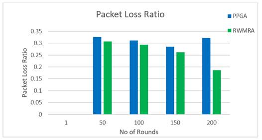
9.3. PLR PACKET LOSS RATIO

Real time network, due traffic or any environmental factors cause packet collision, packet loss ratio can be calculated by

 

 

The quantity of packets sent from source to destination in a regular time interval is shown in Figure 7 and is used to estimate the throughput of the mobile sensor network. It has been described along with the planned Random waypoint mobility Routing's operating philosophy.

Each area head in the Mobile Sensor Network will forward data packets along the best routing path. The Mobile Sensor Network is divided into m regions. After aggregation, these mobile routing nodes will transfer the data to the following region head or BS. In this way, routing region heads receive and control more than 50% of the data transmitted to BS.

Figure 7

                                                               

Figure 7 Packet Loss ratio for time interval T

 

The information received by each region, and it is the case of RWMRA technique, the packets are sent to single or multi hop manner. In regular time interval 20 seconds, the proposed model improves packet delivery ratio 25% approximately. This shows more than 5% increase in energy. Node collision rate is lesser in RWMRA compared with PPGA. This proposed work is improves the PLR.

 

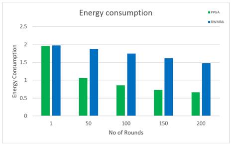
9.4. EC ENERGY CONSUMPTION

Total amount of sensor node energy consumed after completion of each rounds is calculated by,

 

EC =

 

The consumption ratio is high, when the node does not affect by any environments factors. Node Initial energy = 30 J from Figure 4, the number of sensor nodes (along x-axis) is compared with the (along y-axis) to regular time interval T calculate the energy consumption of network.

Figure 8

                                                                

Figure 8 Energy Consumed for time interval T

 

However, it is clear from the graphic that the time interval of 20 seconds out of 120 nodes is shown in RWMRA's proposed mobile sensor network

After all rounds have been completed, it is clear that the energy consumption is 3% lower. These findings demonstrate that the suggested RWMRA demonstrated lifetime performance that was 34% better than PPGA and more than 4 times better than EPFA. Consequently, the required greater performance was achieved.

 

10. CONCLUSION

In this study, Random waypoint mobility routing has been proposed for the enhancement performance packet delivery ratio in MSN. Regions were dynamically divided up in the network field. The centre of the network region was designated as BS. Nearby CHs were able to converse with BS directly while using minimal energy.

The introduction of mobile routing nodes in region 2 increased the network lifetime by conserving node energy as they travelled along the designated path to collect data from region 3's CHs and send it to the BS after aggregating it. In order to send the data packets along the region using Euclidean distance, RWMRA is linked with an angle-based routing. This protocol's goal is to cut down on energy usage and data transmission delays.

Simulations run using MATLAB are used to analyze the performance of RWMRA. The main MSN performance indicators are specified and assessed for a range of sensor node counts, sink speeds, and network sizes. By contrasting our protocol with existing cutting-edge routing methods, the effectiveness and efficiency of our protocol are shown.

The network field can be further divided into more than 200m and introduced with additional nodes, different network topologies, and varying mobility speeds, which will increase throughput. Even while adding several mobile sinks to RWMRA would be simple, maintaining and updating their locations on VS nodes will raise communication overhead. RWMRA can be improved further while maintaining a trade-off between communication overhead and acceptable application delay to meet the issues caused by multiple mobile sinks.

While choosing the head to employ when assessing the routing technique, we take into account the RWMRA parameter. closer to discover the best routing in a sensor network, we also consider additional characteristics.

 

CONFLICT OF INTERESTS

None. 

 

ACKNOWLEDGMENTS

None.

 

REFERENCES

Alagu Pushpa, R., Vallimayil, A., and Sarma Dhulipala, V. R., (2011). International Journal of Communication Network and Security. Impact of Mobility Models on Mobile Sensor Networks, 1(1), 102-106. https://doi.org/10.1109/ICECTECH.2011.5941866.

Almesaeed, R., and Jedidi, A. (2021). Dynamic Directional Routing For Mobile Wireless Sensor Networks. Ad Hoc Networks. Sciencedirect, 110/10230. https://doi.org/10.1016/j.adhoc.2020.102301.

Chatterjee, S., Chakraborty, A., Dey, R., Banerjee, H., Pareek, S., Nayak, S., Gautam, A., Saha, H. N., Neyaz, M., and Dokania, M. (2017). A Load Balanced Routing Protocol For Mobile Sensor Network, 8th Annual Industrial Automation and Electromechanical Engineering Conference (IEMECON). IEEE Publications. https://doi.org/10.1109/IEMECON.2017.8079576.

Hemalatha, S. and Prakash Raj, E. G. D. (2020). Strategic Survey and Analysis of Routing Algorithms for Mobile Sensor Networks. International Journal of Advanced Science and Technology.

Hemalatha, S. and Prakash Raj, E. G. D. (2019). PPGA: Partial-Partitioned Greedy Algorithm for Routing In Mobile Sensor Networks. International Journal of Scientific and Technology.

Hemalatha, S., and Prakash Raj, E. G. D. (2018).Enhanced Greedy Perimeter Forwarding Algorithm for Mobile Sensor Network in Cluster Region. International Journal on Computer Science and Engineering. https://doi.org/10.26438/ijcse/v7i6.115123.

Ma, X., Zhang, X., and Yang, R. (2019). Reliable Energy-Aware Routing Protocol in Delay-Tolerant Mobile Sensor Networks. Wireless Communications and Mobile Computing, 2019, 1-11. https://doi.org/10.1155/2019/5746374.

Murugan, K., and Khan Pathan, A. (2019). A Routing Algorithm For Extending Mobile Sensor Network's Lifetime Using Connectivity and Target Coverage. International Journal of Communication Networks and Information Security (IJCNIS). https://doi.org/10.17762/ijcnis.v11i2.4102.

Sun, Z., Zhao, Guozeng, and Xing, X. (2018). ENCP: A New Energy-Efficient Nonlinear Coverage Control Protocol in Mobile Sensor Networks. EURASIP Journal on Wireless Communications and Networking, 2018(1). https://doi.org/10.1186/s13638-018-1023-7.

Yang, Y., Lee, D.H., Park, M.-S., and In, H. P. (2009). Dynamic Enclose Cell Routing In Mobile Sensor Networks. Dept of Computer Science and Engineering College of Information and Communications Korea University. https://doi.org/10.1109/APSEC.2004.46.