Does Environmental Degradation an Outcome of Economic Development? The role of Financial Development and Energy Consumption

 

S. Maheswaranathan ¹, V. Niranjani ²,  S. Tharshini ³

 

¹ Senior Lecturer in Economics, Faculty of Commerce and Management, Eastern University, Sri Lanka

² Temporary Assistance Lecturer, Department of Economics, Faculty of Commerce and Management, Eastern University, Sri Lanka

³ Development Officer, D.S. Division Eravur Town, Sri Lanka

 

1. INTRODUCTION

Human life has become more luxurious, efficient, and comfortable as a result of globalization and industrialization, but economies are also at risk of increased catastrophe. Environmental deterioration has become a major issue all across the world and it is only increasing worse. A variety of factors, including financial development and energy usage, contribute to environmental degradation.

Environmental degradation has a major issue in the world that adversely affected not only the sustainable economic performance of countries but also affect the health of humans.  Mainly carbon dioxide emissions have widely and significantly contributed to global warming which ultimately has a heinous impact on climate change and increases environmental pollution around the world Arafat et al. (2022) Rafique et al. (2022) Environmental degradation has evolved into a significant issue that affects human health and country’s economic performance in the long term Murshed et al. (2020) Arafat et al. (2022)  According to the environmental Kuznets Curve (EKC) hypothesis, environmental degradation will increase during the early stages of a country’s economic development but will begin to decline after reaching a certain level of industrialization Grossman and Krueger (1995) Allowing to Ozturk and Acaravci (2010) carbon emissions contribute to approximately 60% of total global greenhouse gas emissions. The high level of industrialization, high level of energy consumption, and increasing economic growth rates are some of the reasons for the CO2 emissions contribution. As concluded by Saqib (2022) since the entire global population has been contributing to environmental destruction it become has been exceedingly challenging to maintain economic growth in recent years. Further, effective financial development is expected to have a good atmosphere and contribute to stimulating the economy. Yu and Qayyum (2021) also found stable financial development empowers to implementation of innovative and energy efficient technology that reduces the emission level. In contrast, Tamazian et al. (2009) Charfeddine and Kahia (2019) and Shahbaz et al. (2012) found that financial development stimulates economic development triggering more emissions and severe harm to the environment.  Based on energy management, a country’s real income growth is influenced by energy consumption and increasing manufacturing production leads to increased global warming and carbon footprint Shahbaz et al. (2012) Yang et al. (2021)

Adams and Nsiah (2019) revealed, that both renewable and non-renewable energy sources cause carbon dioxide emissions in the long run. However, the impact of renewable energy on carbon emissions diminishes in the short run. Further, they found a positive relationship between economic growth and environmental degradation. da Silva et al. (2018) discovered that economic growth had a positive effect on renewable energy consumption in emerging countries and Sub-Saharan Africa. In OECD countries economic growth influenced renewable energy consumption positively in the long run but negatively in the short run Alam and Murad (2020) Rahman and Velayutham (2020) found a unidirectional causality in South Asia from economic growth to renewable energy consumption.

If the country consists of a well-established financial system, companies can increase their production by lending loans at a reduced interest rate which facilitates more power usage and increases carbon emissions Bui (2020) Therefore, financial development has a significant impact on the ecosystem by linking with energy and growth. Therefore, the present study aims at examining the impacts of financial development, energy consumption and economic development on environmental degradation in Sri Lanka during 1990 to 2019, for the first time in the literature, using a time series econometric approach of dynamic ARDL simulations that produced reliable and robust results.

This study is organized as follows: Section 2 explains the literature review. Section 3 discusses the data, model, and approach, while the conclusion and recommendation were included in the final section of the study.

 

2. LITERATURE REVIEW

This section attempts to look at previous scholarly work on the relationships between energy consumption, economic development, financial development, and carbon emissions from a variety of perspectives, including life expectancy.

 

2.1. ENERGY CONSUMPTION AND ENVIRONMENTAL DEGRADATION 

Energy consumption and Gross Domestic Product (GDP) per capita are the major contributors to environmental degradation Nurgazina et al. (2021) Shobande and Ogbeifun (2022) Qayyum et al. (2021) Szymczyk et al. (2021) Baydoun and Aga (2021) Energy consumption and technological innovation significantly negative impact on environmental degradation in both the short and long run Qayyum et al. (2021) Atsu et al. (2021) concluded that ICT and fossil fuel consumption plays a significant role to intensify carbon dioxide emissions, whereas renewable energy consumption and financial development reduce carbon dioxide emissions by employing the autoregressive distributed lag (ARDL), dynamic ordinary least squares (DOLS), and fully modified ordinary least squares (FMOLS) method.

Using data from 1997 to 2016 Salari et al. (2021) discovered that energy consumption had a positive impact on environmental degradation. Further, these findings are supported by the EKC hypothesis. Abbasi et al. (2021) examined the energy consumption GDP and CO2 in Pakistan from 1972 to 2018 by adopting the ARDL bound test approach and frequency domain causality approach. They confirmed that energy consumption positively contributed to environmental degradation. Likewise, Su et al. (2021) examined the relationship between CO2, GDP, and energy consumption in Brazil from 1990 to 2018 by using FMOLS, DOLS, and frequency domain causality approaches and portrayed an increase in energy consumption positively contributes to environmental degradation. This finding is supported by other scholarly people Baydoun and Aga (2021) Szymczyk et al. (2021) Ayobamiji and Kalmaz (2020) Usman et al. (2021)

Ozcan et al. (2020) found that economic growth and energy consumption are the leading causes of environmental degradation in OECD countries. Rasool et al. (2020) investigated the curvilinear relationship between pollution and economic growth in India and concluded that energy consumption, economic growth, and financial development have negative environmental consequences from 1971 to 2014. 

 

2.2. ECONOMIC GROWTH AND ENVIRONMENTAL DEGRADATION 

Energy is vital for production activities, which both stimulate economic growth and contributes to environmental degradation. The higher productivity from a product generally leads to significant energy consumption, which further damages the environmental quality by emitting CO2 into the atmosphere.  Baydoun and Aga (2021) confirmed the existence of a strong positive relationship between economic growth and CO2 emissions in GCC countries.  This strong positive relationship between energy consumption, GDP, and CO2 are found by Szymczyk et al. (2021) in OECD countries by analysing the data from 1990 - 2014.

In South Korea, Adebayo et al. (2021) found emissions triggered economic growth while energy consumption mitigated GDP by employing the ARDL, DOLS, and FMOLS approaches from 1965 to 2019. Similarly, Acheampong et al. (2019) discovered that an increase in GDP caused an increase in emissions levels in Australia. Further, Ayobamiji and Kalmaz (2020) found environmental degradation was caused by an increase in economic growth in Nigeria from 1980 to 2017.  

Qayyum et al. (2021) discovered that economic development and urbanization have a positive effect on CO2 emissions in both the short and long run, implying that economic progress and urbanization contribute to rising CO2 emissions in India. Maheswaranathan (2020) found the positive relationship between energy consumption and economic growth in Sri Lanka during 1970- 2017. Using panel ordinary least squares (OLS) technique Salari et al. (2021) showed that GDP had a positive impact on CO2 from 1997 to 2016 in the U.S. Su et al. (2021) findings also supported these findings.

 

2.3. FINANCIAL DEVELOPMENT AND ENVIRONMENTAL DEGRADATION 

Advancements in financial development are critical to reducing environmental degradation Scholars suggest that encouraging financial development benefits firms by removing credit constraints and encouraging investment in environmentally friendly advanced technology Atsu et al. (2021) The absence of environmental policies in financial institutions has resulted in increased CO2 emissions Ameer et al. (2022) According to the studies, financial development, energy consumption, and urbanization are the key drivers of environmental degradation Sharif and Raza (2016) Tamazian et al. (2009) Kasman and Duman (2015) Omri et al. (2015). However, Jalil and Feridun (2011) Baydoun and Aga (2021) Shahbaz et al. (2012) found that financial development reduces energy use and environmental degradation. Further, they explain strong financial development inspires the usage of clean and green technologies in the energy sectors which limits the use of conventional production techniques that contribute to environmental pollution. Qayyum et al. (2021) found a significant positive link between financial development and CO2 emissions in India when applying FMOLS, DOLS, and CCR techniques. Shen et al. (2021) found that financial development has a positive impact on carbon emissions.

Vo and Zaman (2020) identified that financial development whittled down carbon emissions across 101 countries from 1995 to 2018 using the generalized method of moments (GMM). Rjoub et al. (2021) used the Bayer and Hanck co-integration and canonical co-integrating regression to investigate the moderating role of financial development in the determinants of carbon emissions and found that financial development can promote environmental sustainability in Turkey.

Usman et al. (2021) confirmed that financial development contributed significantly to environmental degradation in 15 highest-emitting countries.  employed unrelated regression and GMM approach to examine the impact of financial development and energy consumption on carbon emissions for 128 countries between 1990 and 2017 and found that financial development had a positive impact on carbon emissions. Lv and Li (2021) reviewed the spatial effects of financial development on carbon emissions across 97 countries and found that financial development has a negative effect on carbon emissions from 2000 to 2014.

Shobande and Ogbeifun (2022) discovered that when energy consumption rises, financial development drives carbon emission reductions. Economic expansion, according to Kılavuz and Doğan (2021) has a favourable impact on CO2 emissions. Exponential economic growth and financial development reduce carbon emissions, but moderate economic growth and financial development raise carbon emissions Rajpurohit and Sharma (2020)

 

3. METHODS AND MATERIALS

3.1. DATA, VARIABLES AND THE EXPECTED RELATIONSHIP BETWEEN THE VARIABLES

Table 1 and Equation 1 describes the variables used in this study.  The annual time series data for the variables used for the study were extracted from the World Bank database for the period from 1990 to 2019 other than the energy consumption, which was collected from Total Primary Energy Consumption Quadrillion Btu published by the World Bank. Except for the GDP growth rate and financial development, all the data for the series were transformed into natural logarithms to reduce the Skewness of the distribution and to ensure data normality and linearity except for financial development and GDP annual growth. Since more energy use, whether personal or industrial, discharges more carbon dioxide into the atmosphere, it is expected that there is a positive link between energy consumption and CO2 emissions. GDP, on the other hand, measures the increase in population income over a given year. A rise in income is also expected to increase demand for goods and services that emit carbon dioxide. Similarly, as financial development intensifies, so does the creation of products, resulting in increased carbon emissions into the atmosphere.  

Table 1

Table 1 Description of Variables
Variable	Description	Source
Energy Consumption (EC)	Total Primary Energy Consumption Quadrillion Btu	WDI
Financial Development (FD)	Domestic credit to private sector (% of GDP)	WDI
Environmental Degradation (ED)	CO2 Emissions Mton	WDI
Gross Domestic Product (GDP)	GDP growth (annual %)	WDI
Life Expectancy (LXP)	Average number of years a newborn is expected to live	WDI

 

3.2. MODEL SPECIFICATION

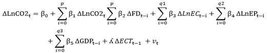
To measure the impact of financial development, energy consumption, and economic growth on environmental degradation, this study employed the following model specification:

 

 =  + FD_t+ LnEC_t +  GDP_t+ LnEP_t + ε₁                   Equation 1

 

where CO_2t is environmental degradation, which is the proxy variable for CO2 Emissions Mton, FD_t is the financial development which is the proxy variable for domestic credit to the private sector the ratio of GDP, ECt is the energy consumption which is the proxy variable for Total Primary Energy Consumption Quadrillion Btu, GDP_t is GDP growth (annual %) and LXP_t is the Life Expectancy.

 

 

 

 

3.3. ANALYTICAL METHOD

This section discusses how the data for this study were analysed. Both exploratory and inferential data analysis techniques were considered analytical tools and exploratory data analysis techniques include scatter plots, confidence ellipses, and kernel fits, whereas inferential data analysis techniques include the unit root test, ARDL bounds test, diagnostic tests, the and Granger causality test.

Since this present study employed time series data to investigate the relationship between economic growth, financial development, and environmental degradation, it is vital to evaluate if the variables are stationary. The Augmented Dickey-Fuller unit root test (ADF) and the Philips–Perron (PP) unit root tests were used in this work to determine the order of integration of the variables. After confirming the order of the variables' integration, the optimum lag length for the model was determined using the Akaike information criterion (AIC) and the Vector autoregression (VAR) technique. Various leg-length criteria have been utilized by different researchers. In this study, however, the Akaike information criterion was employed to select the optimum lag-length model. The long-run relationship between the variables was investigated using the ARDL bounds cointegration technique after determining the appropriate lag length for the model.

 

                                                 Equation 2

 

Where Δ refers to the first difference operator, q, q₁, q₂, q₃ and q₄ are the optimal lag length value. u_t is a random error term, δ0 is constant,    are the long-run coefficients, and   are the short-run coefficients.

After estimating the ARDL model, the following null hypothesis and the alternative hypothesis were tested weather examine the long-term relationship between the variables. The long-run association between the variables was evaluated by relating the calculated F- statistic with the critical values Pesaran et al (2001).

The null hypothesis of no co-integration:

  (There is no co-integration among the variables)

   (There is co-integration among the variables)

When there is long-run co-integration among the variables the following model is estimated.

 

                                                                    Equation 3

 

The ARDL approach was executed after establishing the co-integration test among the variables. Following long-term relations of the variable established, short-term relationship is examined by adopting the Error Correction Model (ECM) Engle and Granger (1987) for the evaluation of short-term coefficients and the Error Correction Term (ECT). The following Equation 4 describes the specification of short-run dynamics of the ARDL model and the error correction model:

    Equation 4               

Where λ denotes the speed of adjustment back to long-run equilibrium following a short-run shock and   denotes the error correction coefficients, which intended to be negative and less than one at the 5% significant to have the long-run equilibrium and  are the short-run dynamic coefficients to equilibrium.

Diagnostic tests, serial correlation, normality, and heteroscedasticity tests, as well as stability tests like CUSUM⁴ and CUSUMSQ, Brown et al. (1975), are performed to validate the model's goodness of fit. If the plots of CUSUM and CUSUMSQ statistics remain within the critical bounds of a 5% significant level, coefficients of the regression are stable, and the null hypothesis can be accepted.

The ARDL co-integration approach concentrates on the existence of the co-integration relationship between variables rather than concentrating on the direction of the variables.  Therefore, Granger (1988) model is employed to examine the causal relationship among the variables. In this study, the Granger causality describes in the following forms:

 

                                                                          

 

                                                                          

 

  (Null Hypothesis)

 

  (Alternative Hypothesis)

 

4. EMPIRICAL FINDINGS AND DISCUSSION

4.1. DESCRIPTIVE STATISTICS

Table 2 shows the summary statistics of the variables used in this study, including mean, maximum, minimum, Skewness, Jarque-Bera, Probability, and Kurtosis values. According to Table 2 the mean of environmental degradation is 2.474, with a range of 1.447 to 3.250. The mean value for financial development, energy consumption, life expectancy, and GDP are 30.53891, -1.572287, 4.293360, and 5.170875, respectively. The skewness values of all variables show that the parameters are normal. The Kurtosis values also reveal that all of the variables are normal. The probability value of the Jarque-Bera illustrates that, unlike GDP, environmental degradation, energy consumption, and financial development conform to normality.

 

 

Table 2

Table 2 Descriptive Statistics
	LnED	FD	LnEC	GDP	LnLEP
Mean	2.474772	30.53891	-1.5723	5.170875	4.293360
Maximum	3.250998	50.01732	-0.9984	9.144572	4.343520
Minimum	1.447030	8.798534	-2.2579	-1.5454	4.237535
Skewness	-0.434101	-0.39232	-0.1733	-0.807	-0.311015
Kurtosis	2.402711	3.103782	2.192915	5.145207	1.404181
Jarque-Bera	1.388162	0.783046	0.964372	9.008286	3.666950
Probability	0.499533	0.676026	0.617432	0.011063	0.159857

 

Figure 1

                                                                            

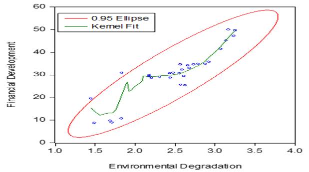
Figure 1 Relationship between Financial Development and Environmental Degradation

 

Figure 2

                                                                            

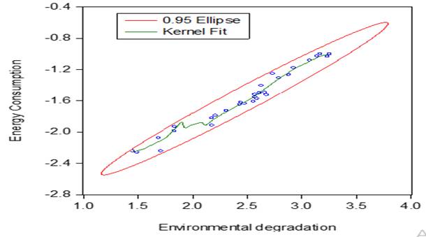
Figure 2 Relationship between Energy Consumption and Environmental Degradation

 

Figure 3

                                                                         

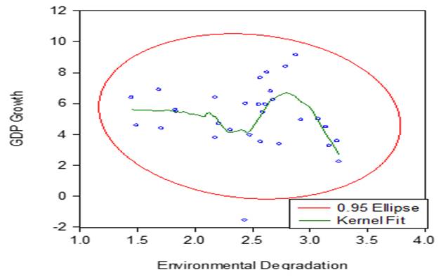
Figure 3 Relationship between GDP Growth and Environmental Degradation

 

Figure 1 and Figure 2 shows the relationship between financial development and environmental degradation and Energy Consumption and Environmental Degradation in Sri Lanka. The Kernel Fit and confidence ellipse curve show the positive relationship of the variables at a 5% confidence level in both figures. At the same time Figure 3 show the negative Relationship between GDP Growth and Environmental Degradation in Sri Lanka during the study period.

 

4.2. UNIT ROOT TEST

The ARDL method can be applied if the series is mixed of I (0) or I (1), without I (2). The ARDL method can perform the unit root test to confirm that none of the series are integrated at I (2). ADF and Perron unit root tests were used in this study to assess the series' integration. As per the table, the parameters are stationary at a mixed level of I (0) and I (1), the ARDL bounds test proposed by Pesaran et al. (2001) is used to investigate the co-integration of CO2 emissions and the explanatory variables.

Table 3

Table 3 Unit Root Test
	Augmented Dickey-Fuller			Phillips-Perron test
Variable	Level (0)	1st Difference (1)	Remarks	Level (0)	1st Difference (1)	Remarks
LnED	-1.455187 (0.5415)	-7.025734 (0.0000)	I (1)	-1.986569 (0.2907)	-7.037489 (0.0000)	I (1)
FD	-0.756047 (0.8165)	-5.645654 (0.0001)	I (1)	-0.756047 (0.8165)	-6.089335 (0.0000)	I (1)
LnEC	-0.986496 (0.7446)	-4.760533 (0.0007)	I (1)	-1.134586 (0.6881)	-4.741258 (0.0007)	I (1)
GDP	-4.009504 (0.0045)		I (0)	-4.009504 (0.0045)		I (0)
LnLEP	-3.997857 (0.0060)		I (0)	-3.997857 (0.0060)		I (0)

 

Table 3 explains the Augmented Dickey-Fuller unit root test statistics and the Phillips-Perron unit root test statistics. Except for life expectancy (LnLEP) and GDP growth rate (GDP), which were stationary at the level I (0), other variables used in this study, such as environmental degradation (LnED), financial development (FD), and energy consumption (LnEC), were stationary at the first difference I(1). This recommends that the hypothesis of non-stationarity is rejected for variables at the level and first difference.

 

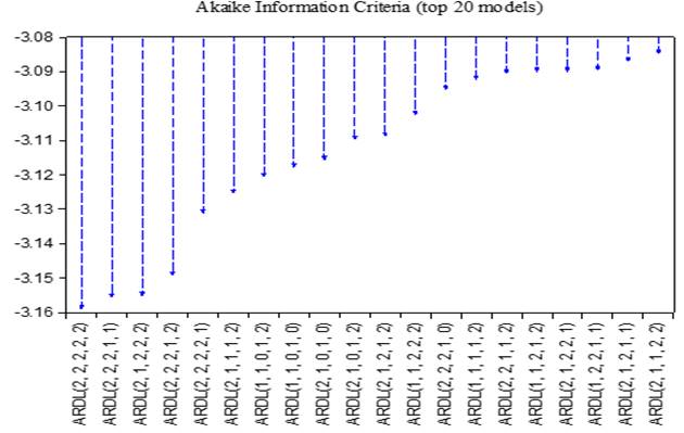
4.3. LAG LENGTH SELECTION

The appropriate lag length selection is vital to perform the ARDL bounds test to examine the co-integration of the variables. Also, valid lag length selection eludes the serial correlation of the error terms. Further, the selection of lag order experienced the calculation of ARDL F-statistic quite sensitive. Furthermore, the lag order would have to be high enough to prevent over-parameter errors in the conditional ECM Naraya (2005) Pesaran (2001). The lag length selection is executed based on Akaike information criterion (AIC) statistics since it is superior for a small sample data set Lutkepohl (2005).   Table 4 shows that the AIC, SIC, and HQ criteria have a lag of 2 when compared to the other criteria. As a result, lag 2 is chosen for the present research based on the Akaike Information Criterion (AIC).

Table 4    

Table 4 VAR order Lag Length Selection
Lag	LogL	LR	FPE	AIC	SC	HQ
0	-34.9866	NA	1.20e-05	2.856186	3.094080	2.928912
1	106.3564	222.1104	3.05e-09	-5.454028	-4.026666	-5.017669
2	162.5368	68.21907*	3.97e-10*	-7.681200*	-5.064370*	-6.881209*

                                                                          

 * indicates lag order selected by the criterion                  

 LR: sequential modified LR test statistic (each test at 5% level)

 FPE: Final prediction error                                

 AIC: Akaike information criterion                       

 SC: Schwarz information criterion                      

 HQ: Hannan-Quinn information criterion

 

 

 

 

 

 

 

 

 

Figure 4

                                                                         

Figure 4 VAR order Lag Length Selection Graph for AIC

 

Figure 4 illustrates the best 20 ARDL models that yielded an Akaike Information Criterion lag length of 2. From these models, the ARDL (2, 2, 2, 2) was considered the best model since it has a low lag length compared with other models to examine the impact of financial development, energy consumption, economic growth, and life expectancy on environmental degradation in Sri Lanka from 1990 to 2019.  

 

4.4. COINTEGRATION TEST

ARDL bounds testing approach was performed after the appropriate lag length section as the next step to test the existence of the long-run relationship between the variables. The findings of the ARDL Bounds Cointegration test are described the following. Table 5

   Table 5

Table 5 ARDL Bounds Cointegration Test
F-statistic	15.30257
Critical Values	Lower Bounds	Upper Bounds
1%	3.29	3.09
5%	2.56	3.49
10%	2.2	4.37

 

The ARDL bounds test results are portrayed in Table 5 The calculated F-statistics value (15.30257) is higher than the critical value at a significance level of 1%. Therefore, the study confirms that in the long run, all variables are cointegrated. Thus, the null hypothesis is not considered, indicating that there is long-term co-integration between economic growth, financial development, energy, consumption, and life expectancy on environmental degradation. 

 

 

4.5. DIAGNOSTICS TESTS

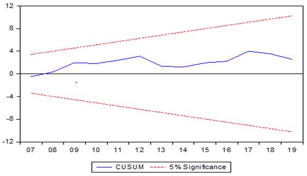
The results of the study are reliable as different diagnostic tests are carried out for both models of the study. The JB and Ramsey RESET test statistics confirm that the error term is normally distributed, and the model is stable as long as the functional form of the model is correct. The model is also free from autocorrelation and heteroscedasticity problems. The stability of the model of the study is also confirmed by the recursive stability check as the CUSUM and CUSUM of squares Figure 5 Figure 6 lines are within the limits. 

Table 6  

Table 6 Diagnostics tests
Diagnostics tests
Test	F-statistic	Prob.
Heteroscedasticity	0.6096	0.8151
Autocorrelation	0.5874	0.5723
Ramsey RESET	0.0067	0.9358
JB Normality	1.5092	0.4701

 

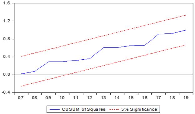
Stability Test

Figure 5 and Figure 6 illustrate the results of model stability of cumulative sum (CUSUM) and cumulative sum of square (CUSUM Q) of recursive residuals for the long-term and short-term parameters. The plot lying between the 5% significant level confirms the stability of the model and further, the model possesses the parameter stability in the short term.

Figure 5

                                                                         

Figure 5 CUSUM test

 

 

 

 

 

 

Figure 6

                                                                            

Figure 6 CUSUM of Squares test

 

The results of the CUSUM and CUSUM squares in Figure 5 and Figure 6 also show that the model is stable at a significance level of 5 %.

 

4.6. ARDL LONG TERM AND SHORT-TERM RESULTS

The results of the ARDL long run and short run estimations are portrayed in Table 7 The findings from the ARDL long run estimation revealed that financial development exerts a positive influence on environmental degradation. This means that by holding other indicators are https://www.thebalance.com/ceteris-paribus-definition-pronunciation-and-examples-3305723  stable, a 0.01443% rise in CO2 emissions is caused by a 1% increase in financial development. The finding is supported by the findings of Qayyum et al. (2021) Shahbaz et al. (2012) Raza et al (2018) Madhu and Giri (2015) Shen et al. (2021) Jianhui Jian et al (2019).

Also, energy consumption exerts a positive and significant impact on environmental degradation in Sri Lanka when applying the data from 1990 to 2019. It means that a 1 percent increase in energy consumption causes to increase the environmental degradation by 0.43425 percent. This finding is consistent with the previous studies of Jianhui Jian et al (2019)

Economic growth exerts a negative and insignificant impact on environmental degradation in Sri Lanka during the study period 1990 to 2019. Life expectancy is, positively connected with the average number of years a newborn is expected to live. It was found that a 1% rise in the average number of years a newborn is expected to live increases the average number of years a newborn is expected to live by 4.674335%. Finally, except for the relationship between GDP and environmental degradation in long term other relationships such as financial development, and energy consumption expose the expected relationship for the sample period.

In the near term, increased energy use and financial development have a positive and significant impact on environmental degradation. Additionally, there is a small but positive correlation between GDP and life expectancy and environmental degradation. This is in line with the author's earlier work Adebayo et al. (2021). Finally, the error correction term (ECT (-1)) of -0.090823 is statistically significant and has the appropriate sign. It suggested, however, that there is a very slow adjustment process in the activities of the power in Sri Lanka since the speed of adjustment to the long run equilibrium is 9 percent.

Table 7

Table 7 ARDL Long Term and Short-Term Results Dependent variable: Environment Degradation (LnED)
Regresses	Long Run Estimators	Short Run Estimators
C	-17.328	-0.02082
	-0.0121	-0.6523
FD	0.01443	0.28963
	-0.0003	-0.0007
LEC	0.43425	0.89369
	-0.04	-0.0188
GDPR	-0.00932	0.00554
	-0.2042	-0.3644
LLEX	4.67433	11.3771
	-0.0034	-0.7381
ECT (-1)		-0.09082
		-0.0088
R-squared                         0.904558
F-statistic                          6.950190
Prob(F-statistic)           0.001263
Akaikeinfo criterion   -2.964519
Schwarzcriterion          -2.196616
Durbin-Watson stat       2.138534

              

The coefficient of determination R2 indicates that 90 percent of the total variation of the environmental degradation in Sri Lanka is jointly explained by financial development, energy consumption, economic growth, and life expectancy. The Akaike information criterion, Schwarz criterion and Hannan-Quinn criterion show that the model is correctly specified. F statistic measuring the joint significance of all regressors in the model is statistically significant at the 5 percent level. Durbin-Watson statistic (2.138534) indicates that the explanatory variables are free from autocorrelation.

 

4.7. Variance Decomposition

Table 8

Table 8 Variance Decomposition of Environmental Degradation (LnED)
Period	S.E.	LCO21	FD	LEC	LLEX	GDPR
1	0.063592	100.0000	0.000000	0.000000	0.000000	0.000000
2	0.087147	63.34697	15.34377	17.87643	0.113571	3.319257
3	0.099585	57.16433	19.86753	17.22161	0.325998	5.420530
4	0.124836	44.00898	25.99019	23.53288	0.457490	6.010468
5	0.144987	38.80134	31.15609	23.46554	0.811623	5.765412
6	0.160118	35.60308	32.21354	24.85920	1.202482	6.121695
7	0.170922	33.34270	33.25638	25.20828	1.627372	6.565269
8	0.179670	31.40159	34.06930	25.56631	1.958319	7.004480
9	0.186668	29.95907	34.96721	25.63054	2.176275	7.266910
10	0.192222	28.95777	35.67011	25.67080	2.280642	7.420675

                                                                                         

Table 8 summarizes the findings of the Variance Decomposition approach, which examines the contribution of one variable due to innovative shocks caused by other variables Pesaran and colleagues (2001). According to Table 8 inventive shocks account for 28.95 percent of environmental degradation, whereas financial development shocks account for 36.67 percent. Furthermore, energy consumption accounts for 25.67 percent of environmental damage. Other variables have been found to have a slight impact on environmental degradation.

 

4.8. GRANGER CAUSALITY

The direction of the dependent variable and independent variables is explained in Table 9 above. The table shows a one-way causal relationship between financial development and energy use as well as between financial development and environmental degradation. However, a bidirectional causal relationship between financial growth and energy use has been discovered from 1990 to 2019 in Sri Lanka.

Table 9

Table 9 Granger Causality
Excluded	Chi-sq	df	Prob.
DFD does not Granger Cause DLCO21	20.07636	2	0.0000
D LCO21does not Granger Cause DFD	3.255536	2	0.1964
D LCO21 does not Granger Cause DLEC	6.227937	2	0.0444
DLEC does not Granger Cause D LCO21	5.793518	2	0.0552
DFD does not Granger Cause DLEC	12.86987	2	0.0016
DLEC does not Granger Cause DFD	3.013158	2	0.2217

 

5. CONCLUSION AND RECOMMENDATION

The present study examines the effect of financial development, energy consumption and economic growth on environmental degradation in Sri Lanka by employing annual time series data from 1990 to 2019. Co-integration of the variables for the long-run and the short-run has been investigated using the ARDL bounds testing approach. The direction of the causality among the variables is analysed by the Granger causality test and the variance decomposition method is employed to check the contribution of one variable due to innovative shocks stemming from other variables.

The ARDL bounds test confirmed the long-run co-integration among the variables which were employed for the present study.  The results validated with the EKC hypothesis mean the level of environmental degradation started to increase with income reached until stabilization point, then started to decrease while income increased. The Granger causality model is applied to investigate the causal relationship among the variables of the study and confirmed that unidirectional causality running from financial development to environmental degradation and financial development to energy consumption. The bidirectional causality was found between environmental degradation and energy consumption. Further, any causality did not find between environmental degradation and economic growth. Variance decomposition analyses were done to investigate the contribution of the variable and concluded that environmental degradation in Sri Lanka (35.67) is commonly described by financial development. Finally, the diagnostic test confirms that the model is free from normality, heteroscedasticity, and autocorrelation. Also, CUSUM and CUSUMQ stability tests confirm the model is stable. Financial innovation should be stimulated throughout the country to meet requirements for long-term development. Further, the development process should be progressed through carbon trading technology, energy structure optimization, and energy consumption efficiency promotion.

 

CONFLICT OF INTERESTS

None. 

 

ACKNOWLEDGMENTS

None.

 

REFERENCES

Abbasi, K. R. Shahbaz, M. Jiao, Z. & Tufail, M. (2021). How do energy consumption, industrial growth, urbanization, and CO2 emissions affect economic growth in Pakistan ? A novel dynamic ARDL simulations approach. Energy, 221, 119793. https://doi.org/10.1016/j.energy.2021.119793

Acheampong, A. O. Adams, S. & Boateng, E. (2019). Do globalization and renewable energy contribute to carbon emissions mitigation in Sub-Saharan Africa ? Science of the Total Environment, 677, 436-446. https://doi.org/10.1016/j.scitotenv.2019.04.353

Adams, S. & Nsiah, C. (2019). Reducing carbon dioxide emissions; Does renewable energy matter?. Science of the Total Environment, 693, 133288. https://doi.org/10.1016/j.scitotenv.2019.07.094

Adebayo, T. S. Awosusi, A. A. Kirikkaleli, D. Akinsola, G. D. & Mwamba, M. N. (2021). Can CO2 emissions and energy consumption determine the economic performance of South Korea ? A time series analysis. Environmental Science and Pollution Research, 28(29), 38969-38984. https://doi.org/10.1007/s11356-021-13498-1

Alam, M. M. & Murad, M. W. (2020). The impacts of economic growth, trade openness and technological progress on renewable energy use in organizations for economic co-operation and development countries. Renewable Energy, 145, 382-390. https://doi.org/10.1016/j.renene.2019.06.054

Ameer, W. Amin, A. & Xu, H. (2022). Does Institutional Quality, Natural Resources, Globalization, and Renewable Energy Contribute to Environmental Pollution in China ? Role of Financialization. Frontiers in Public Health, 10. https://doi.org/10.3389/fpubh.2022.849946

Arafat, W. M. G. Haq, I. U. Mehmed, B. Abbas, A. Gamage, S. K. N. & Gasimli, O. (2022). The Causal Nexus among Energy Consumption, Environmental Degradation, Financial Development and Health Outcome: Empirical Study for Pakistan. Energies, 15(5), 1859. https://doi.org/10.3390/en15051859

Atsu, F. Adams, S. & Adjei, J. (2021). ICT, energy consumption, financial development, and environmental degradation in South Africa. Heliyon, 7(7), e07328. https://doi.org/10.1016/j.heliyon.2021.e07328

Ayobamiji, A. A. & Kalmaz, D. B. (2020). Reinvestigating the determinants of environmental degradation in Nigeria. International Journal of Economic Policy in Emerging Economies, 13(1), 52-71. https://doi.org/10.1504/IJEPEE.2020.106680

Baydoun, H. & Aga, M. (2021). The Effect of Energy Consumption and Economic Growth on Environmental Sustainability in the GCC Countries : Does Financial Development Matter? Energies, 14(18), 5897. https://doi.org/10.3390/en14185897

Bui, D. T. (2020). Transmission channels between financial development and CO2 emissions : A global perspective. Heliyon, 6(11), e05509. https://doi.org/10.1016/j.heliyon.2020.e05509

Charfeddine, L. & Kahia, M. (2019). Impact of renewable energy consumption and financial development on CO2 emissions and economic growth in the MENA region : a panel vector autoregressive (PVAR) analysis. Renewable energy, 139, 198-213. https://doi.org/10.1016/j.renene.2019.01.010

Grossman, G. M. & Krueger, A. B. (1995). Economic growth and the environment. The quarterly journal of economics, 110(2), 353-377. https://doi.org/10.2307/2118443

Jalil, A. & Feridun, M. (2011). The impact of growth, energy and financial development on the environment in China : a cointegration analysis. Energy Economics, 33(2), 284-291. https://doi.org/10.1016/j.eneco.2010.10.003

Kasman, A. & Duman, Y. S. (2015). CO2 emissions, economic growth, energy consumption, trade and urbanization in new EU member and candidate countries : a panel data analysis. Economic modeling, 44, 97-103. https://doi.org/10.1016/j.econmod.2014.10.022 

Khan, S. Khan, M. K. & Muhammad, B. (2021). Impact of financial development and energy consumption on environmental degradation in 184 countries using a dynamic panel model. Environmental Science and Pollution Research, 28(8), 9542-9557. https://doi.org/10.1007/s11356-020-11239-4

Kılavuz, E. & Doğan, İ. (2021). Economic growth, openness, industry and CO2 modeling : are regulatory policies important in Turkish economies ? International Journal of Low-Carbon Technologies, 16(2), 476-487. https://doi.org/10.1093/ijlct/ctaa070

Lv, Z. & Li, S. (2021). How financial development affects CO2 emissions : a spatial econometric analysis. Journal of Environmental Management, 277, 111397. https://doi.org/10.1016/j.jenvman.2020.111397

Maheswaranathan, S. (2020). The Relationship between Electric Power Consumption, Foreign Direct Investment and Economic Growth in Sri Lanka, South Asian Journal of Social Studies and Economics6(1), 21-31. https://doi.org/10.9734/sajsse/2020/v6i130158

Murshed, M. Nurmakhanova, M. Elheddad, M. & Ahmed, R. (2020). Value addition in the services sector and its heterogeneous impacts on CO2 emissions: revisiting the EKC hypothesis for the OPEC using panel spatial estimation techniques. Environmental Science and Pollution Research, 27(31), 38951-38973. https://doi.org/10.1007/s11356-020-09593-4

Nurgazina, Z. Ullah, A. Ali, U. Koondhar, M. A. & Lu, Q. (2021). The impact of economic growth, energy consumption, trade openness, and financial development on carbon emissions : empirical evidence from Malaysia. Environmental Science and Pollution Research, 28(42), 60195-60208. https://doi.org/10.1007/s11356-021-14930-2

Omri, A. Daly, S. Rault, C. & Chaibi, A. (2015). Financial development, environmental quality, trade and economic growth : What causes what in MENA countries. Energy Economics, 48, 242-252. https://doi.org/10.1016/j.eneco.2015.01.008

Ozcan, B. Tzeremes, P. G. & Tzeremes, N. G. (2020). Energy consumption, economic growth and environmental degradation in OECD countries. Economic Modelling, 84, 203-213. https://doi.org/10.1016/j.econmod.2019.04.010

Ozturk, I. & Acaravci, A. (2010). CO2 emissions, energy consumption and economic growth in Turkey. Renewable and Sustainable Energy Reviews, 14(9), 3220-3225. https://doi.org/10.1016/j.rser.2010.07.005

Qayyum, M. Ali, M. Nizamani, M. M. Li, S. Yu, Y. & Jahanger, A. (2021). Nexus between financial development, renewable energy consumption, technological innovations and CO2 emissions: the case of India. Energies, 14(15), 4505. https://doi.org/10.3390/en14154505

Rafique, M. Z. Nadeem, A. M. Xia, W. Ikram, M. Shoaib, H. M. & Shahzad, U. (2022). Does economic complexity matter for environmental sustainability? Using ecological footprint as an indicator. Environment, Development and Sustainability, 24(4), 4623-4640. https://doi.org/10.1007/s10668-021-01625-4

Rahman, M. M. & Velayutham, E. (2020). Renewable and non-renewable energy consumption-economic growth nexus : new evidence from South Asia. Renewable Energy, 147, 399-408. https://doi.org/10.1016/j.renene.2019.09.007

Rajpurohit, S. S. & Sharma, R. (2020). Impact of economic and financial development on carbon emissions : evidence from emerging Asian economies. Management of Environmental Quality : An International Journal. https://doi.org/10.1108/MEQ-03-2020-0043

Rasool, H. Malik, M. A. & Tarique, M. (2020). The curvilinear relationship between environmental pollution and economic growth : Evidence from India. International journal of energy sector management. https://doi.org/10.1108/IJESM-04-2019-0017

Rjoub, H. Odugbesan, J. A. Adebayo, T. S. & Wong, W. K. (2021). Sustainability of the moderating role of financial development in the determinants of environmental degradation: evidence from Turkey. Sustainability, 13(4), 1844. https://doi.org/10.3390/su13041844

Salari, M. Javid, R. J. & Noghanibehambari, H. (2021). The nexus between CO2 emissions, energy consumption, and economic growth in the US. Economic Analysis and Policy, 69, 182-194. https://doi.org/10.1016/j.eap.2020.12.007

Salari, M. Javid, R. J. & Noghanibehambari, H. (2021). The nexus between CO2 emissions, energy consumption, and economic growth in the US. Economic Analysis and Policy, 69, 182-194. https://doi.org/10.1016/j.eap.2020.12.007

Saqib, N. (2022). Asymmetric linkages between renewable energy, technological innovation, and carbon dioxide emission in developed economies: non-linear ARDL analysis. Environmental Science and Pollution Research, 1-15. https://doi.org/10.1007/s11356-022-20206-0

Shahbaz, M. Lean, H. H. & Shabbir, M. S. (2012). Environmental Kuznets curve hypothesis in Pakistan : cointegration and Granger causality. Renewable and Sustainable Energy Reviews, 16(5), 2947-2953. https://doi.org/10.1016/j.rser.2012.02.015

Sharif, A. & Raza, S. A. (2016). The dynamic relationship between urbanization, energy consumption and environmental degradation in Pakistan : Evidence from structure break testing. Journal of Management Sciences, 3(1), 1-21. https://doi.org/10.20547/jms.2014.1603101

Shen, Y. Su, Z. W. Malik, M. Y. Umar, M. Khan, Z. & Khan, M. (2021). Does green investment, financial development and natural resources rent limit carbon emissions ? A provincial panel analysis of China. Science of The Total Environment, 755, 142538. https://doi.org/10.1016/j.scitotenv.2020.142538

Shobande, O. A. & Ogbeifun, L. (2022). The criticality of financial development and energy consumption for environmental sustainability in OECD countries : evidence from dynamic panel analysis. International Journal of Sustainable Development & World Ecology, 29(2), 153-163. https://doi.org/10.1080/13504509.2021.1934179

Shobande, O. A. & Ogbeifun, L. (2022). The criticality of financial development and energy consumption for environmental sustainability in OECD countries : evidence from dynamic panel analysis. International Journal of Sustainable Development & World Ecology, 29(2), 153-163. https://doi.org/10.1080/13504509.2021.1934179

Silva, P. P. D. Cerqueira, P. A. & Ogbe, W. (2018). Determinants of renewable energy growth in Sub-Saharan Africa: Evidence from panel ARDL. Energy, 156, 45-54. https://doi.org/10.1016/j.energy.2018.05.068

Su, Z. W. Umar, M. Kirikkaleli, D. & Adebayo, T. S. (2021). Role of political risk to achieve carbon neutrality: Evidence from Brazil. Journal of Environmental Management, 298, 113463. https://doi.org/10.1016/j.jenvman.2021.113463

Szymczyk, K. Şahin, D. Bağcı, H. & Kaygın, C. Y. (2021). The effect of energy usage, economic growth, and financial development on CO2 emission management : an analysis of OECD countries with a High environmental performance index. Energies, 14(15), 4671. https://doi.org/10.3390/en14154671

Tamazian, A. Chousa, J. P. & Vadlamannati, K. C. (2009). Does higher economic and financial development lead to environmental degradation: evidence from BRIC countries. Energy Policy, 37(1), 246-253. https://doi.org/10.1016/j.enpol.2008.08.025

Usman, M. Makhdum, M. S. A. & Kousar, R. (2021). Does financial inclusion, and renewable and non-renewable energy utilization accelerate ecological footprints and economic growth ? Fresh evidence from the 15 highest emitting countries. Sustainable cities and society, 65, 102590. https://doi.org/10.1016/j.scs.2020.102590

Vo, X. V. & Zaman, K. (2020). Relationship between energy demand, financial development, and carbon emissions in a panel of 101 countries : "go the extra mile" for sustainable development. Environmental Science and Pollution Research, 27(18), 23356-23363. https://doi.org/10.1007/s11356-020-08933-8

Yang, Z. Abbas, Q. Hanif, I. Alharthi, M. Taghizadeh-Hesary, F. Aziz, B. & Mohsin, M. (2021). Short-and long-run influence of energy utilization and economic growth on carbon discharge in emerging SREB economies. Renewable Energy, 165, 43-51. https://doi.org/10.1016/j.renene.2020.10.141

Yu, Y. & Qayyum, M. (2021). Impacts of financial openness on economic complexity : Cross‐country evidence. International Journal of Finance & Economics.