The blind side of a rain gauges network: introductory theoretical approach, with a first example of application

 

Gianmarco Tardivo ¹

 

¹ Unaffiliated, Padova, Italy

 

1. INTRODUCTION

Rain gauge networks are still very important, they are useful in many fields of application even after the advent of weather radars Dervos and Baltas (2024), Abu Salleh et al. (2019). In any case compared to radars they have a continuous measurement system from the point of view of time, although it is, spatially, only punctual Lim, S. (2020) and still represent the first choice in most hydrological applications Dai et al. (2017). In particular, automatic tipping bucket rain gauges (TBRGs) are the most common automatic instrument Dervos and Baltas (2024).

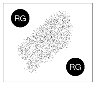
Given the spatial punctuality of the measurements, a network of rain gauges is characterized by the discretion and above all by the finiteness of location points of ground measurements of atmospheric precipitations that can impact the ground on limited areas. It is clear that such impacts can occur completely and precisely in the interspace of the network, i.e., in areas of the surface where the network lies but without measurement points. Rainfall depth measurements from such events will be completely and permanently lost from the network Figure 1 example of impact area between rain gauges.

Figure 1

 

Figure 1 RG: Rain Gauges. White Area Around Rain Gauges: Blind Area of the Network. Dotted Area Inside the Blind Area: Impact Area of an Event Completely Lost by the Network

 

The network therefore has a blind side. Through this dysfunction the network risks losing track of events that could be numerous or individually intense; in any case, they could be significant.

It would be important to take these lost quantities into account, at least to know whether in a more or less dense network, significant quantities of losses can be estimated. A very dense network may not have major losses. But it can also be a competition of climatic, geomorphological and meteorological factors specific to the area in which the network lies, which make the measurements effective also from this point of view (of the loss of measurements), despite the fact that the network does not have a high density of stations.

The temporal resolution Zbynek Sokol et al. (2021) or measurement frequency of the network also has notable importance; this will be particularly highlighted in the "Conclusions" section

In this paper, a theoretical model is proposed, agreeing on equations between the variables involved, which allow a useful interpretation of the problem. These equations make it possible to estimate some hydrological characteristics of precipitation events, in particular those events completely lost by the network measurement system: events with an impact area that is completely embedded in the blind area of the network Figure 1.

Rain gauges are considered the best sources for long-term analysis of precipitation Katharina Lengfeld et al. (2020): it is well known that the associated databases often cover decades of measurements.

In the explanation of the theoretical aspects we proceed from the point of view of the rain gauges-network, i.e., as if we only had a database of rain gauge measurements available. Therefore, without the aid of radar (or remote sensing) data, underlining however that, generally, radar also has its blind side, deducible from a temporal sampling error TSE: Villarini et al. (2008). If the order of magnitude of the temporal resolution Zbynek Sokol et al. (2021) of the rain gauge network were comparable with that of the eventually supplied radar, a spatio-temporal intersection of blindness could occur which would prevent each other's errors from being appropriately corrected. Also taking into account that in this analysis events with a generally small impact area and short-term duration are treated.

It is well known that the measurement errors that characterize a network of rain gauges (for example automatic tipping bucket rain gauges) are many and of various kinds Segovia-Cardozo et al. (2021). The difficulty in their estimation and correction is also well known Segovia-Cardozo et al. (2021). The specific shortcoming addressed in this article, however, seems rather ignored by the literature, especially through the hypotheses of the present analysis, i.e. the absence of data from other types of gauges (e.g. remote sensing instruments), having only data available from the rain gauge network.

The phenomenology of atmospheric events is involved in the study through reasonable physical hypotheses of isotropy and local homogeneity.

The study conducted in this paper is aimed at timeless interpretations of the phenomenon, without therefore analysing its dynamic aspect. The theoretical analysis is set geometrically on a surface, i.e. on a two-dimensional space.

To facilitate the construction of the theoretical model and make statistical applications easier, the rain gauges are thought of as distributed at the points of an averagely regular square mesh network. The edge-size of this mesh however depending on the density of the network.

We will try to establish mathematical relationships between beams of atmospheric events and measured events (i.e. events detected by rain gauges) and not measured events (completely impacting the blind area). These relationships are examined from the point of view of the numerousness, their rainfall depth and the volume they can produce once they reach the ground.

The study highlights the fact that the size of the impact area of events is very important. In order for the impact to have the probability of occurring in the blind area Figure 1, the average impact area must respect some dimensions directly linked to the density of the network in the zone involved.

We can therefore say that, in this context, such events, having an impact area of the order of magnitude the inverse of the network density, can be defined: extremely isolated events (with respect to the local density of the network itself). The higher the network density, the smaller the area of extremely isolated events: this allows the impact areas of such events to be geometrically approximated to compact circular or square areas, consistently with the regular mesh approximation of the network in a specific local density.

This approach is proposed and explained following the subsequent schedule.

Some preliminary hypotheses and useful definitions are given. Some necessary observations are made. Some particular numerical sets are defined to facilitate the description of the methods. Geometric probability methods are applied to obtain the value of the probability that an event can be measured by at most a single rain gauge; this probability turns out to be a function of network density and the extent of the impact area of an event. These functions are crucial for the development of subsequent topics allowing the equations to be built that will be applied in a first numeric example of a real network, to obtain estimates of rainfall depths completely uncaptured by rain gauges. Equations for estimating the number of events falling in the blind area of the network, their rainfall depths and associated volumes are then determined.

In a last supporting paragraph, of non-central importance, some relationships are deduced regarding the average rainfall depths of the three types of bundles discussed: the original bundles of events, generated by the atmosphere; the bundles of events that managed to obtain the measurement of a single rain gauge; the bundles of events that fell in the blind area. These latter relationships are proposed because it is believed they could be a useful mathematical/statistical tool in the possible application of the model to a real network of rain gauges.

In the "Comments and Discussions" section we preferred to proceed initially by describing the phases of a probable application to a DB of real measurements, commenting on the equations that may gradually become involved in the analysis. Assuming a priori that we have the useful parameters available of each of the extremely isolated events that were measured by one and only one rain gauge in the network.

Some important or interesting aspects, theoretical or practical, regarding the defined equations will be discussed.

A first application with empirical analysis of the methods developed here is presented, considering the precipitation data DB of a network in north-eastern Italy as imput. From this first estimate it can be seen that the average annual value of rainfall falling in the blind area of the network around a rain gauge can reach 80% of the average annual total rainfall value measured by the same rain gauge (of which, just under 10% is attributable to the measurements of extremely isolated events). This percentage (80%) seems to be confirmed by the literature Katharina Lengfeld et al. (2020), where an estimate of the amount of hourly heavy events captured by weather radar and not captured by rain gauges can be found. During the present analysis, possible functions are determined which can be assumed as probability distributions for the sizes of the impact areas of the extremely isolated precipitation events taken into consideration. These distributions give much greater probability to smaller impact areas: this will be in favour of a lower loss in terms of rainfall volumes. The purpose of the proposed application example is to obtain a regional average estimate over the entire area covered by the studied network.

 

2. METHODS AND RESULTS (INTRODUCTORY THEORETICAL APPROACH)

2.1. PRELIMINARY HYPOTHESES

In these pages, the character of local homogeneity and isotropy of some target variables such as rainfall depth and number of events is assumed by hypothesis.

Given a zone of the network with density ρ and a bundle of events with average impact area σ, on the zone, it is assumed that the number of events and the rainfall depth of the bundle (or the impacts) are both distributed in a homogeneous and isotropic way (on the zone with density ρ). The adjective "local" refers to the specific density, so that for two distinct densities heterogeneity of the beam can be admitted.

Phenomena will be analyzed in this paper, only from a static point of view and therefore: timeless, not dynamic.

At each point of a geographical surface covered by a network of rain gauges, an average density ρ of these rain gauges can be determined.

Every precipitation event has an impact area on the ground, which will be more or less extensive; based on its extension, this event could be measured in some points by a certain number of rain gauges.

 

2.2. SOME USEFUL DEFINITIONS AND OBSERVATIONS.

The average impact area with the ground of an event will be called section: σ. Since sets of events with the smallest sections that impact the network are considered, it is statistically permissible to attribute an average circular or square section to them. This makes the geometric probabilistic treatment of the topic easier.

Measurement by the rain gauge of the rainfall depth of the event will be called reaction, and therefore a reaction corresponds to the actual “meeting” between an event and the rain gauge.

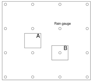
In this paper the flag Extremely Isolated Precipitation Event (EIPE) is given to an event which, once it reaches the ground, is measured by at most a single rain gauge (or which has no reaction at all) Figure 2.

An event that occurs and is not measured by any rain gauge will be called an undetected event (square A of Figure 2).

Figure 2

 

Figure 2 Example of EIPE with Single Reaction (B), and without Reaction (A: Undetected Event). Small Circles Represent Rain Gauges

 

A set of precipitation events, which occur in a certain time and that impact a specific geographical surface, not necessarily measured by a rain gauge, will be called a beam (of events) (In Figure 3, larger circles delimit average impact areas of the events of a beam). An event of a beam will also be called an element of the beam.

Figure 3

 

Figure 3 The Bold Dots Represent Rain Gauges. The Larger Circles Delimit the Approximate Impact Areas of a Fruitful Beam of Section Compatible with the Density of the Network. Bold Circles Represent those Beam Events that were Detected by a Single Rain Gauge

 

From now on we could say a “zone ρ” (or just “ρ”) instead of “a zone with density ρ”. Also, with regard to σ, one can refer directly to a beam of section σ (or just a section σ), meaning: a beam made up of elements of average section σ. Everything will be clear from the context.

When the section σ in the given density ρ can statistically produce single reactions (i.e. reactions with at least one rain gauge, and not more than one) this defines a compatibility relation between σ and ρ. See Figure 3.

 

3. DEFINITION OF SOME SETS: .

A precipitation event with section σ will be intended to be measured at most by a single rain gauge (i.e. producing at most a single reaction), in an area with density σ ≤ ρ^-1. Instead, for example, it will be measured by at least one rain gauge if σ ≥ ρ^-1, and if σ ≥ 4ρ^-1 it will always be measured by at least 2 rain gauges. These properties are clarified better in the section regarding the application of geometric probability.

 defines the set of sections compatible with ρ in the weak sense;  defines the section associated with the density ρ. , with , will identify any discrete and finite subset contained in S(ρ)the cardinality of which will be equal to l, with l∈ℕ.

The sections for which σ ≤  (with ) will be called sections compatible with ρ in the strong sense, called  (note that given  we have that  and if   is sufficiently lower than  it happens that ), With an analogous discrete and finite set, with , with cardinality, also, ∈ℕ. In both cases (compatibility in the weak sense and in the strong sense) the relationship between σ and ρ is obviously symmetrical: we can therefore also say that ρ is compatible with σ (in the weak or strong sense).

In fact, for convenience we also define : this is the set of ρ compatible with σ in the weak sense. We will denote by   a discrete and finite subset of .

We define   the set of ρ compatible with σ in the strong sense;  is a discrete and finite subset of .

For ease of writing we define with  any theoretical continuous set of densities of a hypothetical network, with  corresponding to the maximum density value present in the analyzed network:, any discrete and finite subset of .

The total set of sections compatible (both weakly and strongly) with some ρ of the network can be found to be the following:  where corresponds to the minimum density detected in the network.

Compatibility remains synonymous with the fact that the section in the given density can statistically produce single reactions (i.e. reactions with at least one rain gauge, and not more than one).

It is clear that the beams with a section in  will not be able to produce undetected events and will be called fruitless beams. The fruitful beams (beams capable of producing undetected events) will have a section belonging to  Figure 3. EIPEs can be produced from both fruitless and fruitful beams. However, the  beams (i.e., beams with the average section belonging to ) are made up only of EIPE events, unlike the  beams which also produce not-EIPE events.

EIPEs are therefore the set of events that have become “fruit” (undetected event), or that have led to a single reaction.

 

4. ON THE PROBABILITY THAT AN EVENT WILL GET A SINGLE REACTION (GEOMETRIC PROBABILITY)

It should be noted that the probability with which the number of events of a beam with an average section belonging to translates into the number of single reactions (i.e., the number of impacts on a single rain gauge) will be calculated in a different way from a beam with an average section belonging to S(ρ).

This derives from the fact that in one case we are in the presence of fruitful beams and in the other, instead, of fruitless beams.

To give a simple geometric explanation of the two probabilities just highlighted, we analyze the impact position of an event of section σ that falls on an area with density ρ. The topic is solved with the geometric probability methods Mathai (1999), Klain and Rota (1997) outlined below.

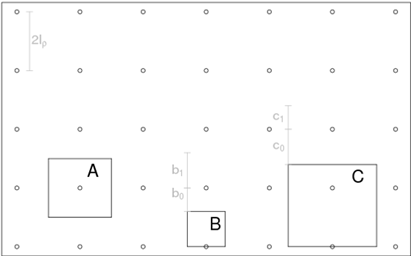
Assuming a square section with sides  (with ) that flows in an averagely regular network of square mesh with sides of length  being the section with side . By following a straight line as in Figure 4, it is noted that through a cyclic distance the section encounters 0, 1 or more rain gauges. The same thing happens when traveling along a straight line perpendicular to the previous one. It must be taken into account that the two perpendicular linear directions analyzed are associated with two marginal distributions of a bivariate variable; these distributions must be considered stocastically independent.

The distances are those described in the following explanations.

1)   The probability of a single reaction in the case S(ρ). See Figure 4 “C”.

Inside an area with density ρ, the possible linear displacement, to obtain a single reaction, of an event with a square section of half-side (or radius if circular section, is the same)  where   is the half-side of the area section  and , is equal to  (Figure 4, c₀) over a total length of , where  is the portion of the linear displacement of the event, within the same area, to obtain a number of reactions strictly greater than 1 (Figure 4, c1). Therefore, the respective linear probabilities are  and , with . It can be deduced that the spatial probability of obtaining only one reaction is equal to .

2)   The probability of a single reaction in the case T(ρ). See Figure 4 “B”.

Inside an area with density ρ, the possible linear displacement, to obtain 0 reactions (an undetected event), of an event with a square section of half-  where   is the half-side of the area section  and , is equal to  (Figure 4, b₀) over a total length of , where  is the portion of the linear displacement of the event, within the same zone, to obtain a single reaction (Figure 4, b1). Therefore, the respective linear probabilities are   and , with . It can be deduced that the spatial probability of obtaining only one reaction is equal to . In this case we found precisely the probability predicted by the elementary and fundamental equations (which are used here from a simplified point of view) of nuclear physics, used (in an obviously more sophisticated form and generally defined in differential terms) within the topic of “scattering”, in particular in the definition of the so-called “cross section” Landau and Lifshitz (1982).

We call  and  single reaction factors (or projection factors) of the beams on the network.

Figure 1

Figure 4 The Small Circles Represent Rain Gauges Inside an Area of Average Density  . . A Is an Event with Section . B Is an Event with Section of Half-Side , with . C Is an Event with Section of Half-Side , With .  and  Identifying the Linear Vertical Displacements (In Succession) Of the Upper Edge of Square B To Obtain 0 Reactions Or 1 Reaction Respectively.  And  Identify the Linear Vertical Displacements of the Upper Edge of Square C To Obtain One Or More Than One Reaction Respectively.

 

NOTE.

Weak compatibility is called weak because the events of such sections have the probability of hitting only one rain gauge, hence the compatibility, but their beams are fruitless, hence the weakness.

NOTE.

The case  is a special case (Figure 4, “A”); it could be considered both as  and as , it is a case of boundary between the two sets; for  we have .  The beams can be considered fruitful beams with 0 fruits (0 undetected events) or they can be considered fruitless beams whose beam elements all completely translate into single reactions, i.e. with no cases where 2 or more rain gauges are hit simultaneously.

 

4.1. ON THE NUMBER OF EVENTS

In the subsequent rows, reasoning about single reactions or rainfall depths can be considered applicable to a single rain gauge or the full set of rain gauges of a ρ-zone.

It is worth specifying that in the following lines, σ generally represents the average section of the beam events and ρ the average density of the rain gauges in the area where the beam impacts. It will become clear when the meaning of the symbols is to be considered different.

In this paper we only analyse reactions that occurred with no more than one rain gauge, that is, we are interested in taking into consideration the rainfall events that can be measured (given the section that characterizes them) by no more than one rain gauge: those that have been defined as EIPE.

From the database of a network of rain gauges (thinking, for example, about a multi-year network of tipping rain gauges with a time-step of a few minutes), for each individual rain gauge, it is possible to collect the number, depths and durations of the single reactions that occurred with the EIPEs.

Calling  the number of these reactions, in order to obtain estimates of event values regarding the blind area of the network, it seems clear that this number must be divided into two components:

 

                                                                                                 (1)

 

 being the number of single reactions with the EIPEs of S(ρ) (called fruitless-EIPEs);  the number of reactions with T(ρ) (fruitful-EIPEs). The analysis of  is important because this number must be subtracted from the total number of single reactions detected by a rain gauge to obtain the fruits (undetected events) of the rain gauge.

Analysis of the fruitful component: .

The single reactions of this component () recorded by a rain gauge can be divided into a number of sections, the beams of which produced such reactions, allowing the following distributional equation:

 

                                                              (2)   

where each of the  () represents the number of reactions had with the beam of section ;  is a relative frequency distribution, and is such that .

The relationship between the number of events of a beam, , of section σ (with σ compatible with ρ in the strong sense) and the number of single reactions is given by the following equation, in which the single reaction factor was calculated previously:

 

 

                   
                                                               (3)

 

which implies .

From here we can immediately write the total expression of and thus obtain a more complete relationship between beams and single reactions:

 

                                                                   (4)

 

which can also be written: , moving from a relation between numerousness (cardinalities) to a relation between surfaces (between strong EIPEs and their reactions).

To have a clearer vision of the relationships between beams and single reactions in the context of fruitful sections ( o ) the following definitions/findings may be useful.

 that represents the overall number of events of beams with all possible sections σ strongly compatible with the density ρ.

 that represents the part of overall reactions (over all ρ densities strongly compatible with σ) obtained from beams of section σ.

, the total number of events of beams of section σ that produced reactions on all densities ρ strongly compatible with σ.

The definition of   introduces one of the main topics of this paper giving mathematical expression to the fruits of the beams E(ρ) (i.e. the undetected events) deducting from the previous equations:

 

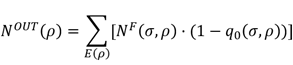                                                                         (5)

 

where = with .

Consequently, the following is also obtained (numerousness balance):

 

                                                                                            (6)

 

From the previous equations we obtain:

 

                                                                      (7)

 

From the latter, the expression of the ratio between fruits and reactions of a strongly compatible beam can be deduced:

 

                                                                                                                                               (8)

 

Analysis of the fruitless component: .

For fruitless sections there exists (as deduced from the previously made statistical-geometric considerations) the following relationship between elements of the beams and their single reactions:

 

                                                                                   (9)

 

with  previously calculated equal to: .

 

4.2. ON THE RAINFALL DEPTHS

Assuming the knowledge of a distribution of rainfall depths across the section values compatible with a given density, it is clear that relationships similar to the case of the analysis on numerousness can be found; still taking into account the previously mentioned hypotheses about homogeneity and isotropy.

The main ones are written formally; the meaning of the symbols can be deduced from the previous lines.

Also in this case, the two types of components, fruitless and fruitful, must be distinguished:

 

                                                                                               (10)

 

The fruitful component, , corresponds to the following summation:

 

                                                                        (11)

 

where each of the   ()  represents the value of rainfall depth measured by the section beam σ, single-reactions in the ρ-density zone;  is a relative frequency distribution, and is such that .

As for the number of events, the relationships also exist for the rainfall depths:

 

                                                                                       (12)

 

and

 

                                                                                    (13)

 

where = represents the depth of rainfall not measured by the rain gauges in the ρ-area; H^. As with the numerousness, also for the rainfall depths a balance equation can be written (rainfall depth balance): .

Even in the case of rainfall depths, as in the case of event-number, we can write:

 

                                                               (14)

 

(with possibly different from , this last defined for the number of events).

For the fruitless component, the following relationship exists between rainfall depth of the elements of the beams and rainfall depth of single reactions:

 

                                                                                         (15)

 

With previously defined.

 

4.3. ON THE UNDETECTED VOLUME

 

                                                                                                 (16)

 

Where  indicates the overall undetected volume matched to the ρ-area.

Hence, the expression of the overall undetected volume over the region covered by the entire network:

 

                                                                         (17)

 

4.2. ON THE AVERAGES OF RAINFALL DEPTHS

From the specific equations of a section strongly compatible with the density, defined for the numerousness and, respectively, the rainfall depths of the beams,  and  (from eq. (3) and similar for H) we can derive the following relationship between the averages of the rainfall depths :

 

                                                                                (18)

 

Where  ;  and .

From the same equalities and eq. (7) and (14), the equality of the following averages can be further deduced:

 

 

                                                        (19)

 

Then, from equation (8) (for ) and from the analogous equation that can be written for  we can deduce the other relations on the averages of the depths for a given density:

 

                                                                                  (20)

 

From an equation identical to equation (8), ,  for N^F and for H^F this other relation is obtained for the beams.

 

                                                                                            (21)

 

Therefore, being able to deduce an important link between the number of events and the relative averages of rainfall depths:

 

                                                                                            (22)

 

still taking eq. (3) into account.

 

From the trivial equation , the following results: (TR-equation); from which, summing over the strongly compatible sections:

 

                                                (23)

 

From definitions (2) and (11) this relationship emerges, , but above all:

 

                                                                            (24)

 

And finally, from the definition of p and P, the following equation is given:

 

                     (25)

 

with .

Considering the set  of the two triples  and considering two distinct elements of ,  and , with  and , (25) can be written like this:

 

                        (26)

 

5. COMMENTS AND DISCUSSIONS

The main purpose of the theory just exposed is to provide tools for the determination (estimation) of,  and

Considering the application of the model to a real case, i.e. having the network's rainfall database available, the variables that can be obtained from these data are: numerousness, rainfall depth and duration of the single reactions. Sections cannot be obtained directly.

It is presumable that to obtain characteristics (at least from a statistical point of view) regarding the sections involved in the phenomenology studied, specific data analyses must be resorted to, with the possible aid of the relationships found in this paper.

The values collected by the DB regarding the single reactions of each rain gauge present in the DB must be subjected to equations (1) and (10). In fact, from these reactions it is necessary to subtract those relating to fruitless beams, thus allowing one to work directly on the single reactions associated with events in the blind zone. From the point of view of both the numerousness and rainfall depth (N and H), the following values are therefore now available: ,  and .

Once this separation has been accomplished, equations (2), (3), (4), (11) and (12) allow one to establish the relationship between the beams of events produced by the atmosphere, and strongly compatible with the densities involved in the network, and the single reactions (fruitful type) just deduced (always, for both N and H).

Equations (5), (6), (7), (8), (13) and (14) involve and statistically define the portions of events not detected by the network; they relate these events with the original beams and the fruitful single reactions deduced from the DB (for both N and H).

The beam events are precisely distributed between undetected events and single reactions (eq. (6) and analogous for H).

Finally, equations (16) and (17) obtain an estimate of the volumes of rainfall not measured by the network, both for each individual density zone and for the region covered by the entire network.

Equations (9) and (15) express the component of the single reactions, concerning the fruitless beams, as a function of the beams with weakly compatible sections.

This component is no less important than the fruitful component, but this paper highlights, in particular, the topics regarding the fruitful component. It remains clear that even for the fruitless component it could be useful to consider a distribution of the single reactions as a function of the sections. But by only having to subtract these reactions from the overall reactions, it might also be sufficient to obtain a synthetic estimate for them, without specifications on the sections (see the application example section). The single reaction factor, , would have the sole purpose of making known the characteristics of the fruitless beams of events, with respect to the single reactions generated by them.

From the structure of the model, considered from a mathematical-statistical point of view, it can be seen that conducting an analysis on raw data or making use of an inferential analysis regarding the distributions p and P would be crucial (see the application example section). The following values would be available at this point: , , , , , etc.

Equations from (18) to (23) relate the number of events to the rainfall depth; these relationships can become useful in the applied phase of the analysis aimed at estimating the p and P distributions. These equations also highlight some aspects of the model from the point of view of the physical hypotheses initially admitted.

The equivalences (19) show, from a statistical point of view, the correspondence of the hypothesis of local homogeneity placed at the foundation of the phenomenological interpretation.

From these equalities, and considering equation (18), it can also be seen that the average of the rainfall depths of all strong single reactions is distributed according to the p distribution (the distribution expected for the numerousness), both for  and for and for .

Equation (23) also characterizes the relationship that exists between the numerousness and depth of rainfall of the single reactions of each section:  holds the factor p and   instead holds P.

The P distribution is presented by relating the inverse of the averages of the rainfall depths of the reactions (equation (24)). Equation (18) corresponds to (24) with the exchange of roles between  and  between  and  and between p and P.

Returning to equations (3) and (12), a brief overview of the single reaction factors is interesting:  and .

The percentage of a beam of section σ spent in reactions in a density ρ varies linearly from 0% to 100% Figure 5, starting from the null section (section to be considered only theoretical) up to  (the section associated with ρ).

Considering sections and densities strongly compatible with each other: for the same density with the same numerousness of beams, a smaller section produces more fruits (and fewer reactions) than a larger section. Two beams with the same section and numerousness produce more fruits (and fewer reactions) in a lower density.

The fruitless part associated with , however, decreases non-linearly from 100% to 0%, from  Figure 5. Assuming for different sections the same number of events (or rainfall depth) of the beams, approximately the single reactions to be subtracted from  (or )  due to the fruitless component, amount to one and a half times those associated with the fruitful component.

 

 

Figure 5

Figure 5 Percentage of the Number of Elements or Rainfall Depth, Of the Beams with A Section Compatible with A Density Ρ. the Left Increasing Line Represents the Percentage That Can Be Deduced with the Single Reaction Factor for the Fruitful Component, While the Right Decreasing Line Concerns the Fruitless Component.

 

The application of the model presented in this paper could be facilitated by the assumption of some general hypotheses.

For example, one of the trivial hypotheses to be admitted could be that of the equal distribution of the single reactions according to the sections; in this way we would admit  or  (indicating with #(-)  the value of the cardinality of a set). Another hypothesis could be the assumption of global homogeneity of the beams; in this way the numerousness and the value of rainfall depth of each ρ-density zone would depend on the area occupied by this density.

From an analysis of the original precipitation data, a linear, increasing or decreasing dependence of the rainfall depth on the section value could be ascertained ascertained (for example , with  and  constant). With this hypothesis (H1) and with the hypothesis of the equal distribution (for example

) An integral solution to the problem could be convenient, noting that, for example, equation (12) in integral form can be written like this:

 

                                                                                     (26)

 

while, from equation (16), the value of the volume lost in a ρ density zone would be the following:

 

                                                                                (27)

 

which, for example, admitting the validity of hypothesis H1 would give the following value of the undetected volume : . Having considered for simplicity , , with , deducing the following rainfall depth balance (): .

In the final section of this paper, a deeper analysis is presented: a first numerical example of application to a database of measurements coming from a real network of 138 automatic tipping rain gauges located in a region in northern Italy.

A note on local homogeneity assumption:

In some geographical-climatic areas, supported by a specific network of rain gauges, situations could arise in which the hypothesis of local homogeneity is not sufficiently satisfied. In this case one of the possible solutions could be to divide the area of a specific density into subareas. This would lead to making the p and P distributions dependent on a third variable that links the specific density zone to its own subzones.

 

6. CONCLUSIONS

This paper provides tools for an average estimate of the number of lost events, their depth and the volumes associated with them. This average can be reduced to an annual average by dividing the overall estimate found by the number of years of the series of measurements analyzed. This average can be further reduced to an aerial average, providing e.g. a density of volume lost per

It is assumed that the results of this paper can be useful in various fields, e.g. in the hydrological field, in the context of hydrological balance calculations Bedient et al. (2019). Generally, this work could be useful in any context in which only rain gauge data is available or in any context in which integration with rain gauge data is deemed necessary. If the network whose data is used is insufficiently dense for the climatic and hydrological context with which we are dealing, an appropriate correction of the precipitation values deduced from the rain gauges could be significant: clearly taking into account the undetected and estimated volumes.

The method also has limitations of applicability. During the analysis it was found out that: the denser the network, the smaller the extent of such non-captured events, in fact the σ_ρ section associated with ρ will be smaller for a denser network. If the network is too sparse compared to the measured territory, the method may not give reliable results. In the extreme case of a single rain gauge, all measured events would be considered EIPE.

It also seems clear that: the higher the network measurement time frequency, the shorter the potentially deductible duration of such events. But it should also be noted that a low measurement frequency could cause significant, even if of short duration, isolated events to be missed.

Table 1 shows a simplified clarifying example. St.1 represents the target station, of which we want to extract the EIPE values. St.2 is the closest station to St.1, followed by St.3 and St.4. It is assumed that the network takes a measurement every 5 minutes. We find an EIPE just as the sum of the measurements at 00:15 and 00:20 time; its overall depth is 1.2 mm (0.8 + 0.4). This event is isolated due to the null value of the depths accumulated by the other stations contemporary to the EIPE found for St.1. It can be seen that if the network measurements instead occurred every 30 minutes, the event found would no longer be isolated since in the 30 minutes of the table the other stations would also have measured rainfall. The EIPE would therefore be undetectable from the coarsest time-resolution of the data.

Table 1. An excerpt of a hypothetical TBRG network DB is represented here. St.1 is the station for which the EIPEs are to be obtained (target station). St.2 is the closest station to St.1, followed by St.3 and St.4. hh:mm is the time format. Assuming that the network takes a measurement every 5 minutes. The measurement values are in mm.

Table 1

Time	Station
	St.1	St.2	St.3	St.4
00:05	0.0	0.4	0.0	0.0
00:10	0.0	1.2	0.0	0.0
00:15	0.8	0.0	0.0	0.0
00:20	0.4	0.0	0.0	0.0
00:25	0.0	0.0	0.6	0.0
00:30	0.0	0.0	1.4	0.0

 

Another problem that would make the application of the present methodologies very difficult would be that of too many missing data in the series: missing data from a station close to the target station makes the identification of EIPEs difficult.

We then want to highlight that in the application of these methodologies, having available for example a database of rainfall measurement values with a time-step of just a few minutes, we realize that the variables that can be deduced directly from this database are limited. They can be for example: single reactions with atmospheric events, the number of such reactions, the durations of the events detected, maximum values and intensities of the events, rainfall accumulations or rainfall depth, etc... The values of sections are not directly deducible from this material. It is assumed that any characteristics can be deduced indirectly, and approximately, through numerical and statistical analyses of the available data, also knowing that an event single-reacting in a ρ zone cannot necessarily have a mean section greater than 4, and in the case of strong compatibility it cannot have a mean section greater than .

It is very important to create a good algorithm for the collection of single reactions: it must take into account the fact that the measurement of 2 simultaneous extremely isolated events that hit 2 rain gauges, at a sufficiently long distance from each other, can be considered 2 distinct single reactions belonging to 2 different rain gauges.

The dynamic aspect of the phenomenon, i.e. the temporal flow, has not been analyzed in this paper; even if the topic would be very interesting, but in preparing for an introductory discussion the dynamic analysis is conveniently postponed to any further in-depth analysis.

Here we only point out that this dynamic aspect is evidently dependent on the measurement frequency of the network, which represents an upper limit of significance for the frequency of the dynamics.

 

 

 

 

7. FIRST APPLICATION EXAMPLE AND EMPIRICAL ANALYSIS

This section describes a first analysis and application of the methods presented here. In particular, from the rainfall depth values of the EIPEs which are obtained from the DB of a real TBRG network, the mean annual rainfall depth of the EIPEs falling in the blind area is deduced.

The TBRG network taken into consideration is that of the Veneto region Tardivo et al.  (2022). In particular, 138 rain gauges are considered, with a series length of 21 years (2000-2020) and a time resolution of 5 min.

Network density spans from 0.0012434 (minimum density) to 0.0161642 (maximum density) stations per km2. The average density of the network () is therefore 0.0087038 stations per km2, from which we can reduce the value of the area of the section associated with  () equal to 114.89235 km² ().

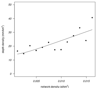
The graph of the mm/km2 values collected by the network-DB for each density zone is represented in Figure 6 (dots in the graph).

The collection of EIPEs in the DB is organized considering not only events that were measured by a single rain gauge in the network, but also those that reacted with multiple rain gauges. In the latter case, if among these reactions there are reactions sufficiently distant from all the others, these single reactions are considered EIPE for these stations, whose measurement is therefore isolated compared to the overall phenomenon. Only 5-minute data with a minimum precipitation value of 0.4 mm are considered.

Looking at formula 10, , the following value in mm of  was obtained from the DB: 352513.6.  

To find the fruits (deductible from ) you need to deduce the  component and subtract it from . To this end, some plausible form of the section distribution must be deduced. It is possible to obtain this distribution by considering equations 12 and 15, which when added together make up ; moving on to the equations in integral form:

 

 

Wanting to obtain a regional average estimate of the value of the annual rainfall depth, in a blind area, attributable to any rain gauge, it is convenient to analyze the curve (dots in Figure 6) ,  being the area of ​​the density zone .

G and therefore F such that

 

 

which can fit are sought.

Some analyses were conducted (which are not reported in this context for brevity) which led to a first choice for  (-indipendent funtion):

 

 

with ,  and  and  such that  is always greater than  on both the intervals  and the linear regression between  and obtains the minimum least squares error Figure 6. In our case:  and

With these parameters the following values are obtained for  and  for various usual statistical tests: .

 Figure 6

Figure 6 Dots: Depth Density of Each Network Density Present in the Rain Gauge Network (). Line:  Deductible From , With , ,  And  Estimated Constants.

 

 is considered as the probability distribution of the sections, where:

 

 

At this point  and .

Numerical results: =17285.86 ; .

equivalence can be assumed by looking for a regional average estimate.

To deduce the estimate of mm associated with the fruits, refer to formulas 13 and 14:

 

 

where  Figure 7: . Numerical results: .

Knowing that the average annual rainfall accumulated by a rain gauge in the network studied here amounts to 1230 mm (), it was deduced that 9.4% of  were mm measured from fruitful beams (), while the estimate of mm falling in the blind area () reaches 83.48% of . From these latest results it can be deduced that the fruitful events detected by the rain gauges represent 10.2% of the total actually fallen Katharina Lengfeld et al. (2020).

Figure 7

Figure 7 Distribution . Where  Spams from  to .

 

Some comments

It is understandable that the distributions to be preferred in this context may have the form

 

 

in fact, for F=, we have that (except for some particular value of n)

 

 

a polynomial of , with  and  parameters dependent on , curves that are well suited for fitting .

Initially analyses were conducted on  (that is, for F with only one addend), obtaining an optimal result for .However, the resulting statistical tests are not as significant as the case presented above: ; standard deviation=In this case corresponds to 8.38% of , and ⁄((number of stations·number of years)) to 45.86% of .

It is expected that by using a 6-parameter , i.e. , even better results can be obtained.

It should be noted that when dealing with this type of function () it is best to use a value greater than zero as the left margin of the set : due to the integral operator. The choice in this paper was for . Figure 7.

Briefly, the results obtained could be explained by noting that: 9.4% of corresponds to 115.62 mm i.e. 1114.38 mm of are not H^R; 83.48% of corresponds to 1026.8 mm, so it can be conjectured that the total average annual rainfall falling around a rain gauge in the region reaches about 2250 mm.

It is important to note that the previously estimated value of 83.48% of must be associated with the distribution calculated for the sections. Therefore, the calculation of the volumes lost by the network is mainly linked to the smaller sections in favour of a reduction in lost volumes.

It may be interesting to know that the average duration of EIPEs numerically captured by network data is 7.2 minutes; the maximum duration is 2.5 hours (values dependent on the threshold parameter chosen, safely, for the determination of EIPE: at least 0.4 mm for a 5-minute datum). The monthly distribution obtained from the entire network is a bi-modal distribution, with the most significant peak in the month of May and a second peak in November.

 

CONFLICT OF INTERESTS

None. 

 

ACKNOWLEDGMENTS

Thanks to Prof. Vincenzo Bixio (University of Padua) for the encouragement and advice given to me. Thanks to Prof. Antonio Berti of the University of Padua for his important advice.

 

REFERENCES

Abu Salleh, N. S., Mohd Aziz, M. K. B., & Adzhar, N. (2019). Optimal Design of A Rain Gauge Network Models: Review Paper. Journal of Physics: Conference Series, 1366(1), 012072. https://doi.org/10.1088/1742-6596/1366/1/012072

Bedient, P. B., Huber, W. C., & Vieux, B. E. (2019). Hydrology and Floodplain Analysis (6th ed.). Pearson.

Dai, Q., Bray, M., Zhuo, L., Islam, T., & Han, D. (2017). A Scheme for Rain Gauge Network Design Based on Remotely Sensed Rainfall Measurements. Journal of Hydrometeorology, 18(3), 363–379. https://doi.org/10.1175/JHM-D-16-0136.1

Dervos, N. A., & Baltas, E. (2024). Development of Experimental Low-Cost Rain Gauges and Their Evaluation During A High-Intensity Storm Event. Environmental Processes. https://doi.org/10.1007/s40710-024-00686-7

Klain, D. A., & Rota, G. C. (1997). Introduction to Geometric Probability. Cambridge University Press.

Landau, L. D., & Lifshitz, E. M. (1982). Course of theoretical physics: Vol. 1: Mechanics.

Lengfeld, K., Becker, A., Kirstetter, P.-E., Fowler, H. J., Yu, J., Flamig, Z., & Gourley, J. (2020). Use of Radar Data for Characterizing Extreme Precipitation At Fine Scales and Short Durations. Environmental Research Letters, 15(8), 10. https://doi.org/10.1088/1748-9326/ab98b4

Lim, S. (2020). A Novel Electromagnetic Wave Rain Gauge and Its Average Rainfall Estimation Method. Remote Sensing, 12(21), 3528. https://doi.org/10.3390/rs12213528

Mathai, M. (1999). An Introduction To Geometrical Probability: Distributional Aspects With Applications. Statistical Distributions & Models with Applications: Vol.1.

Ochoa‐Rodriguez, S., Wang, L.-P., Willems, P., & Onof, C. (2019). A Review of Radar‐Rain Gauge Data Merging Methods and Their Potential for Urban Hydrological Applications. Water Resources Research, 55, 6356–6391. https://doi.org/10.1029/2018WR023332

Segovia-Cardozo, D. A., Bernal-Basurco, C., & Rodríguez-Sinobas, L. (2023). Tipping Bucket Rain Gauges in Hydrological Research: Summary on Measurement Uncertainties, Calibration, and Error Reduction Strategies. Sensors, 23, 5385. https://doi.org/10.3390/s23125385

Segovia-Cardozo, D. A., Rodríguez-Sinobas, L., Díez-Herrero, A., Zubelzu, S., & Canales-Ide, F. (2021). Understanding the Mechanical Biases of Tipping-Bucket Rain Gauges: A Semi-Analytical Calibration Approach. Water, 13(16), 2285. https://doi.org/10.3390/w13162285

Sokol, Z., Szturc, J., Orellana-Alvear, J., Popová, J., Jurczyk, A., & Célleri, R. (2021). The Role of Weather Radar in Rainfall Estimation and its Application in Meteorological and Hydrological Modelling—A Review. Remote Sensing, 13(3), 351. https://doi.org/10.3390/rs13030351

Tardivo, G., Bixio, V., & Bixio, A. C. (2022). A New Method of Identifying An Appropriate Distance Between Independent Extreme Annual Rain Events for a 5-min time Resolution Precipitation Data Network. Theoretical and Applied Climatology, 149, 169–183. https://doi.org/10.1007/s00704-022-04043-2

Villarini, G., Mandapaka, P. V., Krajewski, W. F., & Moore, R. J. (2008). Rainfall and Sampling Uncertainties: A Rain Gauge Perspective. Journal of Geophysical Research, 113, D11102. https://doi.org/10.1029/2007JD009214

Yoon, S. S., Phuong, A. T., & Bae, D. H. (2012). Quantitative Comparison of the Spatial Distribution of Radar and Gauge Rainfall Data. Journal of Hydrometeorology, 13(6), 1939–1953. https://doi.org/10.1175/JHM-D-11-066.1