Modified Inverse Generalized Exponential Distribution: Model and Properties

 

Lal Babu Sah Telee ¹, Vijay Kumar ²

 

¹ Assistant Professor, Department of Management Science, Nepal Commerce Campus, Tribhuvan University, Kathmandu, Nepal

² Professor, Department of Mathematics and Statistics, Deen Dayal Upadhyaya, Gorakhpur University, Gorakhpur, India

 

1. INTRODUCTION

Use of probability model is not limited to statistics only. Statistics has broad application in all the fields of study like applied science, management and economics etc. Since probability distribution has numerous use and applications, it is being modified and generalizing day by day. Probability distribution helps to simulate the real life conditions and to analyze, interpret, and summarize the real life data precisely and effectively and economically in very less time. In literature many new probability models are available that are formulated based on our present requirement of the data analysis. These techniques of introducing new distribution may be by adding some extra parameters to distribution, merging the distribution or inverting the variables etc. These methods make new distribution more flexible and useful than the existing distributions. Literature contains various models for studying the nature and potentiality of the data; still we need new models to explain the new emerging data more precisely. That is in all the cases, classical techniques are not effective as the new distributions. New family of distributions play important role to generalize different models by compounding to well known distribution for introducing suitable models having extra features and properties to handle the variety of data used in theory as well as in practical life Usman et al. (2017)

 Availability of statistical models for studying statistical data is not limited. It is getting introduced new model frequently that can explain various type of data with more precise results. This research is focused on construction of new parametric statistical model. One of methods of getting new model is by introducing extra parameters to existing distribution such as Weibull and exponential family of distribution Marhall & Olkin (1997). Extension of Lomax distribution applying family of Marshall and Olkin model Ghitany et al. (2007) is available in literature.  McDonald Lomax model Lemonte & Cordeiro (2013) has been obtained by Lomax distribution. Power Lomax distribution containing three constants is more flexible than existing Lomax distribution. This model has inverted bathtub as well as increasing and decreasing bathtub hazard rate function Rady et al. (2016).  Model defined has increasing, decreasing and bathtub shaped hazard curve. Exponentiated Weibull Lomax distribution is formulated using exponentiated Weibull-G-family Hassan & Abd-Allah (2018). By taking alpha as an exponent, a new distribution called alpha power inverted exponential was introduced by Ceren et al. (2018) by use of inverted exponential model. Lomax random variable was used as generator by Ogunsanya et al. (2019) in formulating Type III Odd Lomax exponential model. Compounding of inverted Lomax model with odd generalized exponential model results a new distribution called Odd generalized exponentiated Inverse Lomax model given by Maxwell et al. (2019). Lomax exponential distribution has increasing and decreasing hazard rate given by Ijaz & Asim (2019) which was formulated using Lomax distribution. Similarly, inverse Lomax- exponentiated G- family Falgore & Doguwa (2020) is based on Inverse Lomax distribution as generator.

In real life, numerous life time variables are available that may have shape of bathtub hazard rate function. There are many models in literature having bathtub shaped hazard rate curve also. We can get modification of Weibull distribution to get many modified models. Expression below is Weibull distribution having two parameters.

 

 

The hrf of the above model is not bathtub. Many modifications have been performed on this model resulting new model having bathtub hrf. Exponentiated Weibull model introduced by Mudholkar & Srivastava (1993) is well known modification of Weibull distribution. Lai et al. (2016) introduced new lifetime distribution using suitable limits on beta integrated distribution as

 

 

Alqallaf & Kundu (2020); has introduced inverse generalized exponential distribution having two parameters having CDF and PDF as

 

 

 

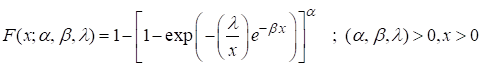
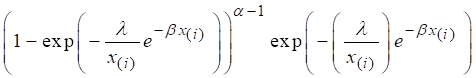
We can add an extra parameter α to modify Inverse generalized exponential distribution as to get new distribution called Modified Inverse Generalized Exponential (MIGE) Model. The cdf and pdf of MIGE model can be given as

 

               

and

 

 

The whole study is studied dividing in different section. First section is introductory where introduction and literature review is mentioned. In second section model formulation and some important properties are mentioned. Next section contains the parameter estimation techniques, Application to real data set and Model comparison. Final section is the conclusion of the study.

 

2. Model Analysis

Modified Inverse Generalized Exponential (MIGE) distribution:

A three parameters MIGE distribution has CDF as,             

 

                            (1)

 

The PDF MIGE distribution can be expressed as,

 

     (2)

 

The Reliability:

Reliability function of MIGE is           

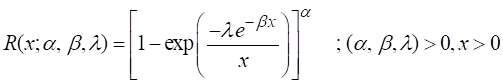                        (3)

 

Hazard rate of model:

Expression (4) is the hazard rate function of the model

 

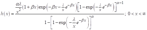                            (4)

 

Reverse hazard function:

The reverse hazard function of MIGE is,

 

    (5)      

 

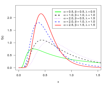
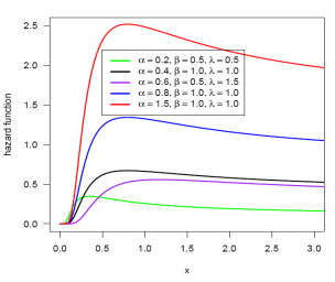
Figure 1 displays hazard rate curve and pdf curve of MIGE with different parameters. From pdf plot it is clear that the density plot for different values of parameter are of different shape. Hazard rate curve is increasing and decreasing or inverted bathtub shaped based on set of parameters.

Figure 1

   

Figure 1 PDF and HRF plots of MIGE Distribution

 

Cumulative hazard rate:

Cumulative hazard rate of the MIGE is

 

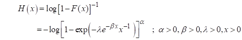                        (6)

 

The Quantile function:

The Quantile function is given by

 

 

Generation of random deviate:

Let u follows uniform distribution then generation of random deviate of MIGE is,

                                   (7)

 

 

We have also defined skewness as well as kurtosis based on quantiles Al-saiary et al. (2019) as,

            and

 

Coefficient of kurtosis Moors (1988) and Al-saiary et al. (2019) is

 

          

 

3. Methods of estimation

This section includes some methods of parameter estimation of the proposed model.

Method of Maximum Likelihood Estimation (MLE)

Here, ML estimators (MLE's) of the MGIE model are estimated by using MLE method. Let  be a randomly selected sample of size ‘n’ from MGIE then the log density function can be written as,

 

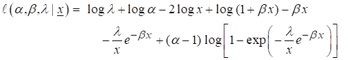
 MIGE has likelihood function as  

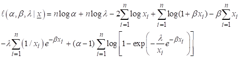                            (8)

 

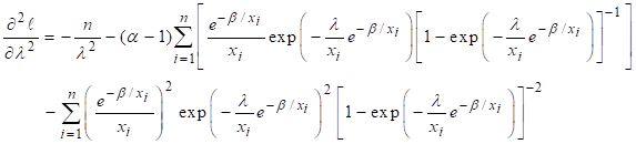
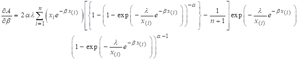
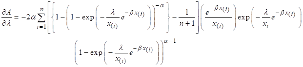
Finding first order derivatives of (8) with respect to constantans

 

      

     

    

   

         

 

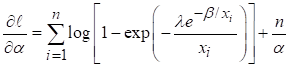
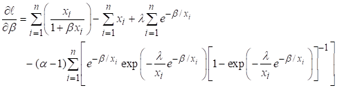
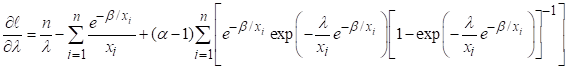
Equating  and performing simultaneous calculations for the α. β, and λ we get the ML estimators of the MIGE   model. But normally, it is not possible to solve non-linear equations mentioned above. Much computer software is available for solving such equations.  Let  is parameter vector and is MLE of  as then the asymptotic normality results in. 

 

                                                (9)

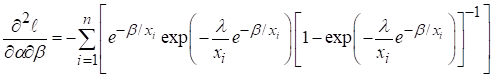
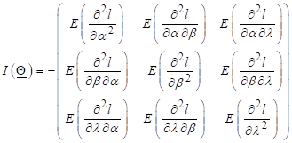
Since may not be known practically, so it will be worthless that the MLE has an asymptotic variance. Let  is observed fisher information matrix of information matrix  such as

 

                              (10)

 

Newton-Raphson method may be used for optimization that will give the observed information matrix. Expression (11) is the variance covariance matrix.

 

                                                     (11)       

 

Also, 100(1-b) % CI for parameters of MIGE   is determined by taking as the upper percentile of the standard normal variate.

 

 

.

 

Estimation by least square (LSE)

Constants α, β, and λ of MIGE distribution and can be determined by minimizing the function (12) also as

 

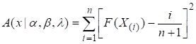                                                                           (12)

 

Suppose  denotes the CDF of the ordered statistics. Let  is a random sample with n items from F (.) is taken The LSE of α. β, and λ respectively, can be determined by minimizing the function (13) as

 

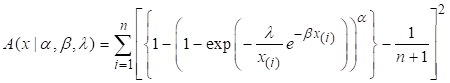                                  (13)

 

Performing partial derivative of (13) with respect to constants as,

 

   

To find the weighted LSE of the function we have minimized the expression below with the parameters to be estimated.

 

          

 

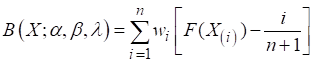
where w_i is weights and has value as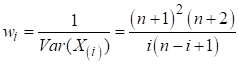 

 

By minimizing the function (14) we can get weighted least square estimation,

 

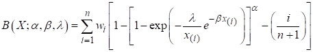                   (14)

 

Estimation using Cramer- von Mises method

This method of estimating constants α, β, and λ are determined using minimization of the function

 

 

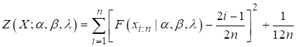
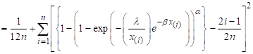                                                (15)

 

First order partial derivatives are,

 

 

                  

       

    

 

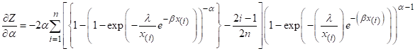
Solving above partial derivatives setting to zero we will get the CVM estimators of the proposed model MIGE.

 

4. Application to Real Dataset

We have presented here a real data. Data is strength data mentioned by Bader & Priest (1982) measured in GPA (Giga Pascal, GPA = KN/mm2, Kilo Newton / square mm.   Data is of single carbon fibers that were tested under tension at gauge lengths of 20 mm and 50 mm. Following is set of data used for the analysis:

1.312, 1.314, 1.479, 1.552, 1.803, 1.861, 1.865, 1.944, 1.958, 1.966, 1.997, 2.006, 2.535, 2.021, 2.027, 2.055, 2.063, 2.684, 2.098, 2.140, 2.179, 2.224, 2.240, 2.253, 2.270, 2.272, 2.274, 2.301, 2.359, 2.382, 2.426, 2.435, 2.478, 2.490, 2.514, 2.554, 2.566, 2.570, 2.586, 2.629, 2.633, 2.642, 2.648, 2.697, 2.726, 2.773, 2.800, 2.809, 2.818, 2.821,2.848, 2.880, 2.954, 3.012, 3.067, 3.084, 3.090, 3.096, 3.128, 3.233, 3.433, 3.585, 1.700.

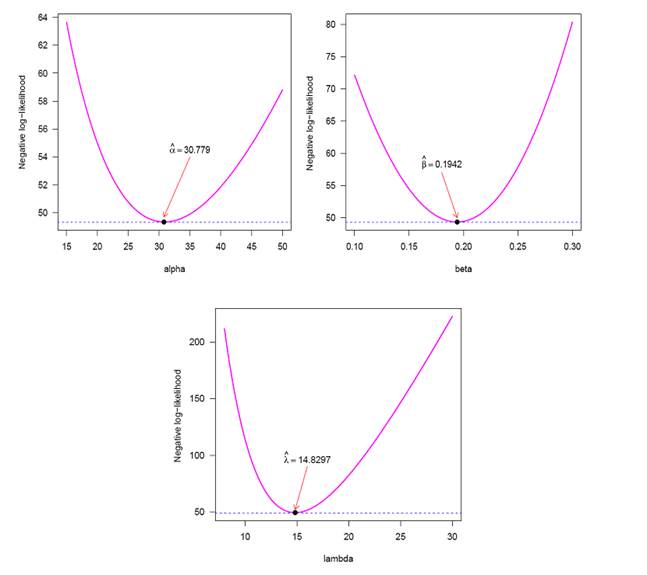
Log-likelihood functions profile for the parameters is in Figure 2 to show the uniqueness of ML estimates.

Figure 2

Figure 2 Log-Likelihood Profile Function

 

Here we have used R programming [R Core Team, 2018] and function optim () to estimate and analyze the parameter values. Value of negative Log-Likelihood is l = -49.3373. MLE’s with their standard errors of parameters are tabulated in Table 1.

Table 1

Table 1 MLE of Parameters and SE
Parameter	MLE	SE
α	30.7790	0.303686
β	0.19420	0.002357
λ	14.8297	1.067448

 

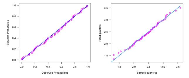
The graph of PP plot and QQ plot are in Figure 3 indicating that validation of the model is justified

Figure 3

Figure 3 PP Plot (Left) and QQ Plot (Right) of Model

 

The estimated value of the parameters of MIGE and their corresponding log-likelihood, AIC, BIC, CAIC, and HQIC calculated and tabulate in Table 2.

Table 2

Table 2 Parameters and Information Criteria Values of Model
Methods				LL	AIC	BIC	CAIC	HQIC
MLE	30.7790	0.1942	14.8297	-49.3373	104.6746	111.3769	105.0438	107.3336
LSE	14.8035	0.3295	16.9123	-49.6935	105.3869	112.0893	105.7562	108.0460
CVE	10.7064	0.4326	19.5468	-50.0715	106.1431	112.8454	106.5123	108.8021

 

Goodness of fit of the model is checked using three methods. We have found the test like KS, W and A² statistic with their corresponding p-value taking the estimated parameter values by MLE, LSE and CVE estimation methods and are presented in Table 3.

Table 3

Table 3 Test Statistics Values Using KS, W and A2 and p-Values
Method	KS (p - Value)	W (p - Value)	A2 (p -Value)
MLE	0.0467(0.9982)	0.0265(0.9868)	0.2227(0.9829)
LSE	0.0443(0.9993)	0.0205(0.9967)	0.2453(0.9728)
CVE	0.0464(0.9984)	0.0207(0.9965)	0.2921(0.9438)

 

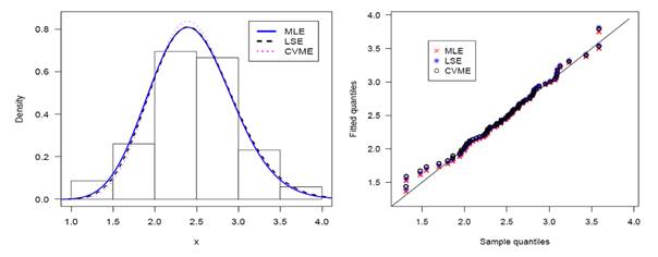
Figure 4 displays histogram versus density function under fitted distributions It also shows fitted quantile versus sample quantile under estimation techniques.

Figure 4

Figure 4 Histogram Versus Fitted Pdf (left) and Fitted Quantile Versus Sample Quantile in Right Side of Estimation Methods MIGE.

 

5. Model Comparison

Applicability testing of MIGE is presented in this section. We have compared the potentiality of the proposed model by comparing this model with other four well known distributions. These distributions are Modified Weibull (MW) Distribution, Generalized Exponential Extension (GEE.) distribution, Weibull Extension (WE) distribution, and Generalized Exponential (GE) distribution. Information criteria values are presents in Table 4. Results shows that defined model fit data better compare to model taken in consideration.

Table 4

Table 4 Information Criteria Values with Log Likelihood Values
Distribution	ll	AIC	BIC	CAIC	HQIC
MIGE	-49.3373	104.6746	111.3769	105.0438	107.3336
MW	-49.6017	105.2033	111.9056	105.5725	107.8623
GEE	-49.6465	105.2930	111.9954	105.6623	107.9521
WE	-50.7239	107.4479	114.1502	107.8171	110.1069
GE	-54.6205	113.2409	117.7091	113.4227	115.0136

 

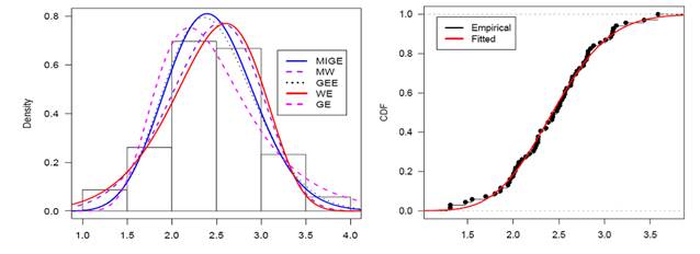
Histogram and the fitted pdf for proposed model as well as the competing models are mentioned in Figure 5. It also includes the fitted cdf and the empirical cdf of the model.

 Figure 5

Figure 5 The Histogram and the Fitted Pdf of Models in Left Side & Empirical Cdf with Estimated Cdf in Right Side of MIGE Model.

 

Goodness-of-fit of the MIGE distribution with other four competing model used earlier by other researchers are compared also. We have also tabulated the value of KS, AD and CVM statistic using R function in Table 5. It is found from calculation that the MIGE smaller value of the test statistic with maximum p-value compared to other

These evidences helped us to finalize that the MIGE gets well fit and produce more regular & valid results from other distributions used for testing.

Table 5

Table 5 Statistics and p Values for Goodness-of-Fit
Models	KS (p-Value)	W (p-Value)	A2 (p-Value)
MIGE	0.0467(0.9982)	0.0265(0.9868)	0.2227(0.9829)
MW	0.0542(0.9873)	0.0326(0.9677)	0.2717(0.9577)
GEE	0.0559(0.9823)	0.0413(0.9279)	0.2924(0.9436)
WE	0.0647(0.9348)	0.0568(0.8357)	0.4431(0.8046)
GE	0.0949(0.5629)	0.1603(0.3603)	1.1235(0.2983)

 

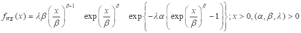
Models taken for Comparison:

Models and pdf are given below

1)    Modified Weibull

The density function of Modified Weibull (MW) model Lai et al. (2003).

 

 

 

2)    Generalized Exponential Extension

Model is introduced by Lemonte (2013) having three parameters is

 

 

 

3)    Weibull Extension

Weibull extension by Tang et al. (2003) has pdf

 

 

 

4)    Generalized Exponential

Gupta & Kundu (1999) introduced this model with pdf

 

 

 

The empirical CDF curve with estimated fitted CDF curve of the model MIGE in Figure 6

Figure 6

Figure 6 Fitted Versus Empirical Distribution Curve of MIGE Model

 

6. Conclusion

Study is based on formulation of new probability model called Modified inverse Generalized Exponential distribution. Some statistical properties and their expressions are derived here. Pdf curve shows that the model is skewed and non normal in nature. Hazard rate curve is monotonically increasing and inverted bathtub shaped. Parameters of the model are estimated using three methods of estimation and the applicability of model is checked using a real data set. For validity testing P-P, Q-Q and fitted versus empirical distribution curves are plotted. For model comparisons, four existing models are considered and some information criteria values are also mentioned. It is found that model fits data better compared to considered model. To test the goodness of fit three well known methods are used. All the computations and the graphical measurement are performed using r programming. The proposed model will play a significant role in studying the different data sets more precisely and will help researcher for the further study of the probability models.

 

CONFLICT OF INTERESTS

None. 

 

ACKNOWLEDGMENTS

None.

 

REFERENCES

Al-saiary, Z. A., Bakoban, R. A., & Al-zahrani, A. A. (2019). Characterizations of the Beta Kumaraswamy Exponential Distribution. Mathematics, 8(1), 23. https://doi.org/10.3390/math8010023.

Alqallaf, F. A., & Kundu, D. (2020). A Bivariate Inverse Generalized Exponential Distribution and its Applications in Dependent Competing Risks Model. Communications in Statistics-Simulation and Computation, 1-18. https://doi.org/10.1080/03610918.2020.1821888.

Bader, M., & Priest, A. (1982). Statistical Aspects of Fiber and Bundle Strength in Hybrid Composites. In : Hayashi, T., Kawata, S. and Umekawa, S., Eds., Progress in Science and Engineering Composites, ICCM-IV, Tokyo, 1129-1136.  

Ceren, Ü. N. A. L., Cakmakyapan, S., & Gamze, Ö. Z. E. L. (2018). Alpha Power Inverted Exponential Distribution : Properties and Application. Gazi University Journal of Science, 31(3), 954-965.  

Falgore, J. Y., & Doguwa, S. I. (2020). Kumaraswamy-Odd Rayleigh-G Family of Distributions with Applications. Open Journal of Statistics, 10(04), 719. https://doi.org/10.4236/ojs.2020.104045.

Ghitany, M. E., Al-Awadhi, F. A., & Alkhalfan, L. (2007). Marshall-Olkin Extended Lomax Distribution and its Application to Censored Data. Communications in Statistics-Theory and Methods, 36(10), 1855-1866. https://doi.org/10.1080/03610920601126571.

Gupta, R. D., & Kundu, D. (1999). Theory & Methods : Generalized Exponential Distributions. Australian & New Zealand Journal of Statistics, 41(2), 173-188. https://doi.org/10.1111/1467-842X.00072.

Hassan, A. S., & Abd-Allah, M. (2018). Exponentiated Weibull-Lomax Distribution : Properties and Estimation. Journal of Data Science, 16(2), 277-298. https://doi.org/10.6339/JDS.201804_16(2).0004.

Ijaz, M., & Asim, S. M. (2019). Lomax Exponential Distribution with an Application to Real-Life Data. PloS one, 14(12). https://doi.org/10.1371/journal.pone.0225827.

Lai, C. D., Jones, G., & Xie, M. (2016). Integrated Beta Model for Bathtub-Shaped Hazard Rate Data. Quality Technology & Quantitative Management, 13(3), 229-240. https://doi.org/10.1080/16843703.2016.1180028.

Lai, C. D., Xie, M., & Murthy, D. N. P. (2003). A Modified Weibull Distribution. IEEE Transactions on Reliability, 52(1), 33-37. https://doi.org/10.1109/TR.2002.805788.

Lemonte, A. J. (2013). A New Exponential-Type Distribution with Constant, Decreasing, Increasing, Upside-Down Bathtub and Bathtub-Shaped Failure Rate Function. Computational Statistics & Data Analysis, 62, 149-170. https://doi.org/10.1016/j.csda.2013.01.011.

Lemonte, A. J., & Cordeiro, G. M. (2013). An Extended Lomax Distribution. Statistics, 47(4), 800-816. https://doi.org/10.1080/02331888.2011.568119.

Marhall, A.W., & Olkin, I. (1997). A New Method for Adding a Parameter to à Family of Distributions with Application to the Exponential and Weibull Families. Biometrika, 84(3). https://doi.org/10.1093/biomet/84.3.641.

Maxwell, O., Friday, A. I., Chukwudike, N. C., Runyi, F., & Bright, O. (2019). A Theoretical Analysis of the Odd Generalized Exponentiated Inverse Lomax Distribution. Biom Biostat Int J, 8(1), 17-22. https://doi.org/10.15406/bbij.2019.08.00264.

Moors, J. (1988). A Quantile Alternative for Kurtosis. The Statistician, 37, 25-32. https://doi.org/10.2307/2348376.

Mudholkar, G. S., & Srivastava, D. K. (1993). Exponentiated Weibull Family for Analyzing Bathtub Failure-Rate Data. IEEE transactions on reliability, 42(2), 299-302. https://doi.org/10.1109/24.229504.

Ogunsanya, A. S., Sanni, O. O., & Yahya, W. B. (2019). Exploring Some Properties of Odd Lomax-Exponential Distribution. Annals of Statistical Theory and Applications (ASTA), 1, 21-30.  

Rady, E. H. A., Hassanein, W. A., & Elhaddad, T. A. (2016). The Power Lomax Distribution with an Application to Bladder Cancer Data. SpringerPlus, 5(1), 1-22. https://doi.org/10.1186/s40064-016-3464-y.

Tang, Y., Xie, M., & Goh, T. N. (2003). Statistical Analysis of a Weibull Extension Model. Communications in Statistics-Theory and Methods, 32(5), 913-928. https://doi.org/10.1081/STA-120019952.

Usman, M., Shaique, M., Khan, S., Shaikh, R., & Baig, N. (2017). Impact of R&D Investment on Firm Performance and Firm Value : Evidence from Developed Nations (G-7). Revista de Gestão, Finanças e Contabilidade, 7(2), 302-321.