ON THE LANZHOU INDEX OF GRAPHS
Qinghe Tong
1![]()
![]() ,
Chengxu Yang 2
,
Chengxu Yang 2![]()
![]() , Wen Li 2
, Wen Li 2![]()
![]()
1 School of Mathematics and Statistics,
Qinghai Normal University, Xining, Qinghai 810008, China
2 School of Computer, Qinghai Normal
University, Xining, Qinghai 810008, China
|
|
|
ABSTRACT |
|
|
Let |
|||
|
Received 29 October 2022 Accepted 30 November 2022 Published 10 December 2022 Corresponding Author Chengxu
Yang, cxuyang@aliyun.com DOI10.29121/granthaalayah.v10.i11.2022.4916 Funding: This research
received no specific grant from any funding agency in the public, commercial,
or not-for-profit sectors. Copyright: © 2022 The
Author(s). This work is licensed under a Creative Commons
Attribution 4.0 International License. With the
license CC-BY, authors retain the copyright, allowing anyone to download,
reuse, re-print, modify, distribute, and/or copy their contribution. The work
must be properly attributed to its author.
|
|||
|
Keywords: Lanzhou Index, Silicate Network, Graph
operation |
|||
1. INTRODUCTION
In this paper, we consider simple, connected, and finite graphs. For a vertex ![]() ,
the number of all edge incidents with
,
the number of all edge incidents with ![]() is denoted by
is denoted by ![]() ,
the maximum (minimum) degree of
,
the maximum (minimum) degree of ![]() is denoted by
is denoted by ![]()
Moreover, we let
![]() and
and ![]() ,
,![]() .
.
The topological index is very useful in chemistry, its
value is related to the molecular structure-activity of the compound. The first
Zagreb index ![]() and the second Zagreb
index
and the second Zagreb
index ![]() ,
introduced by Kazemi in Kazemi
and Behtoei (2017), are defined as
,
introduced by Kazemi in Kazemi
and Behtoei (2017), are defined as
![]()
![]()
Furtula and Gutman in Furtula
and Gutman (2015) introduced the
forgotten index of ![]() ,
which is defined by
,
which is defined by
![]()
After that, Vukičević et al. Vukičević et al. (2018). introduced an index named by Lanzhou index, which is defined as
Let ![]() =
= ![]() be the line graph of
be the line graph of ![]() .
The vertex of corresponds to the edge of
.
The vertex of corresponds to the edge of ![]() .
Two vertices of
.
Two vertices of ![]() are adjacent if and only if the corresponding
edge of
are adjacent if and only if the corresponding
edge of ![]() is adjacent. Then we have
is adjacent. Then we have ![]() .
Line graphs are widely used in the field of chemistry. For example, Nadeem
studied
.
Line graphs are widely used in the field of chemistry. For example, Nadeem
studied ![]() and
and ![]() indices of the line graph of the wheel,
tadpole in paper Nadeem
et al. (2015). Randić found that the connectivity index
of a line graph in some molecular graph is highly correlated with some
physicochemical properties. Gutman further proposed the application of line
graphs in physical chemistry. All this mean that in the field of topology, line
graph is extremely important in the study of chemistry and physics. By
definition of line graph, we have the following observation. From the
definitions, the following observation is immediate.
indices of the line graph of the wheel,
tadpole in paper Nadeem
et al. (2015). Randić found that the connectivity index
of a line graph in some molecular graph is highly correlated with some
physicochemical properties. Gutman further proposed the application of line
graphs in physical chemistry. All this mean that in the field of topology, line
graph is extremely important in the study of chemistry and physics. By
definition of line graph, we have the following observation. From the
definitions, the following observation is immediate.
2.1. Results for line graphs
Observation 1. Let ![]() be
a graph, for
be
a graph, for ![]() ,
and
,
and ![]() ,
we have
,
we have
![]() and
and ![]() .
.
Theorem 2.1. Vukičević et al. (2018). Let ![]() be a connected graph of order
be a connected graph of order ![]() .
Then we have
.
Then we have ![]() .
The inequality is satisfied if and only if
.
The inequality is satisfied if and only if ![]() is
either complete or empty graph.
is
either complete or empty graph.
Theorem 2.2.
Let ![]() be a
connected graph with order
be a
connected graph with order ![]() and
and ![]() . Then
. Then
![]()
With right equality holding if and only if and only if ![]() is a regular graph
and the lower bound is sharp.
is a regular graph
and the lower bound is sharp.
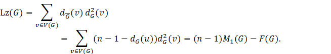
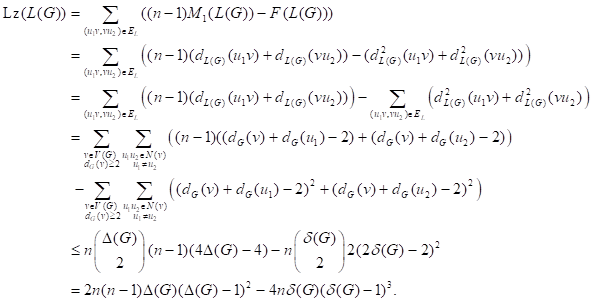
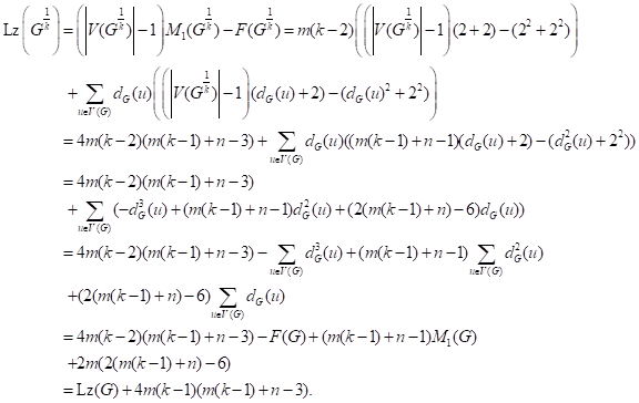
Proof. For the up bound, by
definition of Lanzhou index, we have
With equality holds if and only if ![]() is a regular graph.
is a regular graph.
In addition, for
the lower bound, from Theorem 2, it follows that ![]() .
Let
.
Let ![]() is
is ![]() or
or ![]() or star graph
or star graph ![]() ,
it follows that
,
it follows that ![]() is an empty graph or a complement graph, from
theorem 2, we have
is an empty graph or a complement graph, from
theorem 2, we have![]() .
So, the lower bound is sharp.
.
So, the lower bound is sharp.
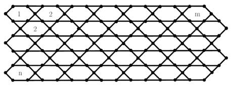
2.2. Results for line graph of graphene sheet
Graphene ![]() is a 2-dimensional layer of pure carbon. Line
graph of graphene
is a 2-dimensional layer of pure carbon. Line
graph of graphene![]() is shown below in Figure 1
is shown below in Figure 1
Figure 1
|
Figure 1 |
Theorem 2.3. Let ![]() are two integers,
are two integers, ![]() ,
and let
,
and let ![]() be a molecular graph of graphene with
be a molecular graph of graphene with ![]() rows and
rows and ![]() columns. Then
columns. Then
Proof. For ![]() , we have
, we have ![]() ,
,
![]() ,
,
![]() ,
and
,
and ![]() .
Let
.
Let ![]() .
From the definition of Lanzhou index, we have that
.
From the definition of Lanzhou index, we have that
Similarly, for ![]() ,
we have
,
we have ![]() ,
,![]() ,
,
![]() ,
and
,
and ![]() .
Let
.
Let ![]() .
Hence
.
Hence
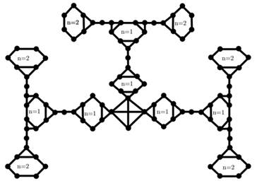
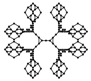
2.3. Results for line graph of DENDRIMER STARS
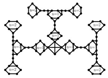
Nanostar dendrimers are generally synthesized by divergent
or convergent methods. It is a kind of hyperbranched nanostructures. ![]()
![]() and
and ![]() are the line graph of three dendrimers and
widely appear in drug structure, see Figure 2, Figure 3, Figure 4.
are the line graph of three dendrimers and
widely appear in drug structure, see Figure 2, Figure 3, Figure 4.
Figure 2
|
Figure 2 Line Graph of Nanostar Dendrimer |
Figure 3
|
Figure 3 Line Graph of Nanostar Dendrimer |
Figure 4
|
Figure 4 Line Graph of
Nanostar Dendrimer |
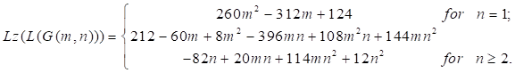
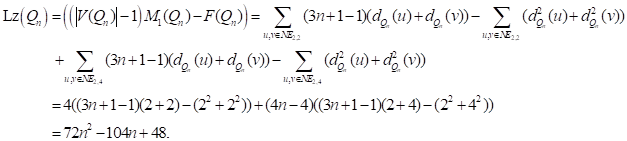
Theorem 2.4. Let ![]() are two integers. Then the Lanzhou index of
line graphs of three infinite classes
are two integers. Then the Lanzhou index of
line graphs of three infinite classes ![]() ,
,
![]() and
and ![]() of dendrimer stars are
of dendrimer stars are
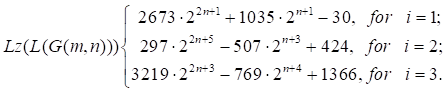
Where ![]() is the number of steps
of growth of these three families of dendrimer stars.
is the number of steps
of growth of these three families of dendrimer stars.
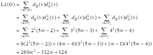
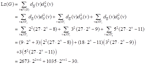
Proof. For ![]() ,
we have
,
we have ![]() ,
,
![]() ,
,
![]() ,
and
,
and ![]() .
Let
.
Let ![]() .
We have
.
We have
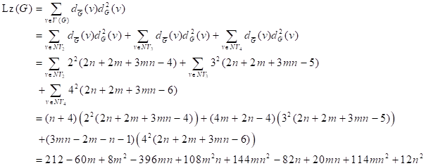
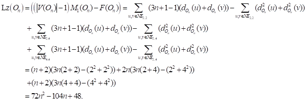
![]() Similarly, for
Similarly, for ![]() ,
we have
,
we have ![]() ,
,
![]() ,
,
![]() and
and ![]() .
Let
.
Let ![]() .
Then we have
.
Then we have
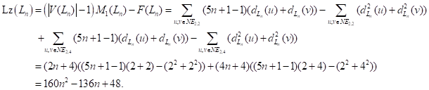
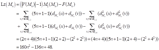
For ![]() ,
we have
,
we have ![]() ,
,
![]() ,
,
![]() , and
, and ![]() .
Let
.
Let ![]() .
By the definition of Lanzhou index, we have
.
By the definition of Lanzhou index, we have

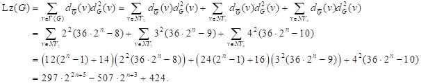
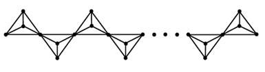
3. Results for CHAIN SILICATE NETWORKS GRAPH
In this section, we consider a family of chain silicate
networks. This network is denoted by ![]() and is obtained by arranging
and is obtained by arranging ![]() tetrahedral linearly, see Figure 5.
tetrahedral linearly, see Figure 5.
Figure 5
|
Figure 5 |
We refer the reader to article Kazemi
and Behtoei (2017) for some aspects of
the parameters of silicate networks. Obviously, for any silicate networks ![]() ,
, ![]() and
and ![]() .
.
Theorem 3.1. Let ![]() be a positive integer,
for an n-long silicate networks
be a positive integer,
for an n-long silicate networks ![]() ,
we have
,
we have ![]()
Proof. Obviously, ![]() .
Note that
.
Note that ![]() is consist of n tetrahedrons which connected
by linear chains. Then we have
is consist of n tetrahedrons which connected
by linear chains. Then we have ![]() and
and ![]() .
Let
.
Let ![]() ,
,
we
get
Define the honeycomb network as![]() .
. ![]() is number of layers
from the center to the boundary in
is number of layers
from the center to the boundary in ![]() . We use a honeycomb network to constructe the silicate
network
. We use a honeycomb network to constructe the silicate
network ![]() by placing silicon
ions on all the vertices of
by placing silicon
ions on all the vertices of ![]() , and dividing the edges and placing oxygenions on the new
vertices, last placing oxygenions at the pendent vertices, where the silicate
network defined as
, and dividing the edges and placing oxygenions on the new
vertices, last placing oxygenions at the pendent vertices, where the silicate
network defined as ![]() .
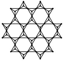
When
.
When ![]() , the silicate network is as follow.
, the silicate network is as follow.
Figure 6
|
Figure 6 |
Obviously, for the silicate networks ![]() , we have
, we have![]() and
and ![]() . The set of edges can decompose as three
types:
. The set of edges can decompose as three
types:
Type (1): ![]()
Type (2): ![]()
Type (3): ![]()
Clearly, we have ![]() .
.
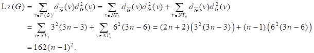
Theorem 3.2. For ![]() ,
the Lanzhou index of hexagons with size
,
the Lanzhou index of hexagons with size ![]() is
is
![]()
Proof.
For ![]() , we have
, we have ![]() ,
, ![]() and
and ![]() . Let
. Let ![]() . By the definition of Lanzhou index, we have that
. By the definition of Lanzhou index, we have that
4. RESULTS FOR SIERPIńSKI GRAPHS
Graphs are widely
used in topology, psychology, and probability Hinz and Schief (1990), Kaimanovich (2001), Klix and Goede (1967).The sierpiński graphs ![]() was introduced by
Pisanski et al. in Pisanski and Tucker (2001).
was introduced by
Pisanski et al. in Pisanski and Tucker (2001).
Let ![]() be
the vertex set of
be
the vertex set of ![]() ,
, ![]() ,
, ![]() . The edge
. The edge ![]() is between two vertices
is between two vertices ![]() and
and ![]() . If there is an integer
. If there is an integer ![]() such that
such that
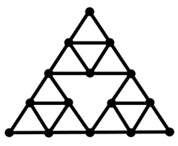
The Sierpiński
graph ![]() is shown in Figure 7.
is shown in Figure 7.
Theorem 4.1. The Lanzhou index of Sierpiński
graph ![]() (also named the Tower of Hanoi with n disks) (
(also named the Tower of Hanoi with n disks) (![]() )
is
)
is ![]() .
.
Proof. Let ![]() . Obviously, the degree of vertex
. Obviously, the degree of vertex ![]() is either 2 or 3. It
is clear that
is either 2 or 3. It
is clear that ![]() and
and ![]() . Then
. Then
The
Sierpiński gasket graphs are extended versions of the Sierpiński
graph. In 2008, Alberto and Anant introduced Sierpiński gasket graph Teguia and Godbole (2006). The sierpiński gasket ![]() is obtained by shrinking all bridge edges of
is obtained by shrinking all bridge edges of ![]() . Sierpiński gasket
. Sierpiński gasket ![]() is shown in Figure 8.
is shown in Figure 8.
Figure 7
|
Figure 7 |
Figure 8
|
Figure 8 |
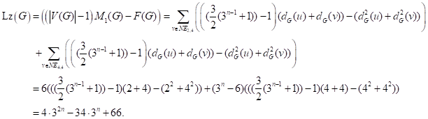
Theorem 4.2. The Lanzhou
index of Sierpiński gasket graph ![]()
![]() is
is
![]()
Proof. In Sierpi´nski gasket graph ![]() ,
,
![]() ,
,
![]() , and the set of edges can decompose as two
types:
, and the set of edges can decompose as two
types:
Type (1): ![]()
Type (2): ![]()
Clearly, we have ![]() .
.
Let ![]() ,
by the definition of Lanzhou index, for
,
by the definition of Lanzhou index, for ![]() , we have
, we have ![]() ,
,
![]() .
. ![]() . Then we have
. Then we have
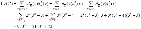
Theorem 4.3.
The Lanzhou index
of Sierpiński gasket graph ![]()
![]() is
is
![]()
Proof, there are ![]() vertices in
vertices in ![]() . The number of
. The number of ![]() degree vertex is
degree vertex is ![]() , and the number of
, and the number of ![]() degree vertex is
degree vertex is ![]() . Next, we consider the vertex in the complement graph
of
. Next, we consider the vertex in the complement graph
of ![]() . In
. In ![]() ,
the number of
,
the number of ![]() degree vertex is
degree vertex is ![]() , and there are
, and there are ![]() vertices with degree
vertices with degree ![]() .
Note that
.
Note that ![]() and
and ![]() .
Let
.
Let ![]() .
Then we have
.
Then we have
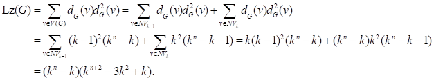
The Sierpiński Gasket Rhombus of level ![]() is defined by
is defined by ![]() , which obtained by identifying the
edges in two copies of
, which obtained by identifying the
edges in two copies of ![]() along one of their sides and
along one of their sides and ![]() Sierpiński Gasket Rhombus
Sierpiński Gasket Rhombus ![]() show in Figure 9.
show in Figure 9.
Figure 9
|
Figure 9 Sierpiński
Gasket Rhombus |
Theorem 4.4.
If ![]() is a Sierpiński Gasket Rhombus graph.
Then
is a Sierpiński Gasket Rhombus graph.
Then
![]() .
.
Proof. Note
that ![]() ,
,
![]() ,
, ![]() ,
, ![]() ,
, ![]() , and
, and ![]() . Let
. Let ![]() and
and ![]() , clearly,
, clearly, ![]() .
Therefore, we have
.
Therefore, we have
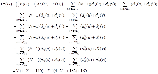
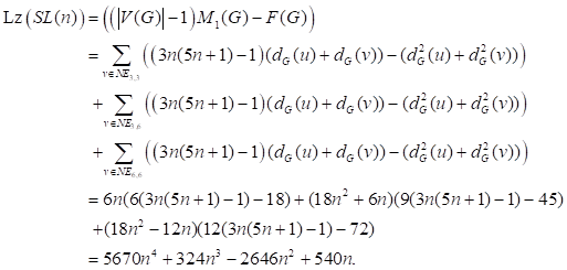
5. LANZHOU INDEX OF CACTUS CHAINS
NETWORKS
The Cactus chain is a simple connected graph. Husimi and Riddell first studied the Cactus graph in Husimi (1950). These graphs are widely used in many fields such as the theory of electrical and communication networks Zmazek and Zerovnik (2005). and in chemistry Zmazek and Zerovnik (2003).
Theorem 5.1. The Lanzhou index of different types of Cactus graphs.
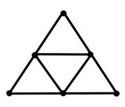
Use ![]() represent the chain triangular graph (See Figure 9). Then
represent the chain triangular graph (See Figure 9). Then ![]() .
.
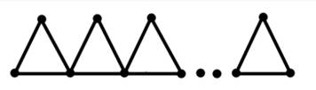
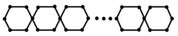
Use ![]() represent the
para-chain square cactus graph (See Figure 10). Then
represent the
para-chain square cactus graph (See Figure 10). Then ![]() .
.
Use ![]() represent the
para-chain square cactus graph (See Figure 11). Then
represent the
para-chain square cactus graph (See Figure 11). Then ![]() .
.
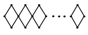
Use ![]() represent the
Ortho-chain graph (See Figure 12).Then
represent the
Ortho-chain graph (See Figure 12).Then ![]()
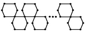
Use ![]() represent the para-chain hexagonal cactus
graph (See Figure 13). Then
represent the para-chain hexagonal cactus
graph (See Figure 13). Then ![]() .
.
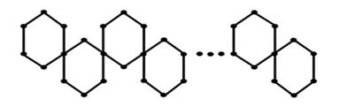
Use ![]() represent the
Meta-chain hexagonal cactus graph (See Figure 14). Then
represent the
Meta-chain hexagonal cactus graph (See Figure 14). Then ![]() .
.
Figure 10
|
Figure 10 |
|
Figure
11 |
Figure 12
|
Figure 12 |
Figure 13
|
Figure 13 |
Figure 14
|
Figure 14 |
Figure 15
|
Figure 15 |
Proof.
1) Note
that ![]() ,
,
![]() ,
,
![]() ,
and
,
and ![]() .
Therefore, we have
.
Therefore, we have
2) Note
that there are four edges with end-vertex of degree 2. Also there are ![]() edges with end-vertex of degree 2 and 4. So we have
edges with end-vertex of degree 2 and 4. So we have ![]() ,
, ![]() and
and ![]() .Therefore, we have
.Therefore, we have
3) Note
that there are ![]() edges with end-vertexs
of degree 2, there are
edges with end-vertexs
of degree 2, there are ![]() edges with end-vertexs
of degree 2 and 4, and there are
edges with end-vertexs
of degree 2 and 4, and there are ![]() edges with end-vertexs
of degree 4. Then we have
edges with end-vertexs
of degree 4. Then we have ![]() ,
,
![]() ,
,
![]() and
and ![]() .Therefore, we have
.Therefore, we have
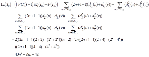
4) There
are ![]() edges with end-vertex of degree 2, there are
edges with end-vertex of degree 2, there are ![]() edges with end-vertex
of degree 2 and 4, and there are
edges with end-vertex
of degree 2 and 4, and there are ![]() edges with end-vertex of degree 4. Then we have
edges with end-vertex of degree 4. Then we have![]() ,
, ![]() ,
,
![]() and
and ![]() .
Therefore, we have
.
Therefore, we have

6) Since
![]() ,
,
![]() and
and ![]() . Then, we have
. Then, we have
6. RESULTS FOR SOME OPERATIONS
For any integer ![]() , the k-subdivision of
, the k-subdivision of ![]() is denoted by
is denoted by ![]() which is constructed by replacing each edge of
which is constructed by replacing each edge of
![]() with a path of length
with a path of length ![]() . Then, we have following result about the Lanzhou index of
k-subdivision of graph
. Then, we have following result about the Lanzhou index of
k-subdivision of graph ![]() .
.
Theorem 6.1. Let ![]() be a graph with
order
be a graph with
order ![]() size
size ![]() ,
, ![]() .
For every
.
For every ![]() .
We have
.
We have
![]() .
.
Proof. There are ![]() edges with end-vertex
of degree 2 and
edges with end-vertex
of degree 2 and ![]() .
Also, there are
.
Also, there are ![]() edges with end-vertex of degree 2 and 2.
Therefore, we have
edges with end-vertex of degree 2 and 2.
Therefore, we have
By the proof of Theorem 13, we get Observation as below.
Observation 2. Let ![]() . Then we have
. Then we have
![]() .
.
We next describe some common binary operations defined on
graphs. In the following definitions, let ![]() and
and ![]() are two graphs with disjoint vertex sets. The
join
are two graphs with disjoint vertex sets. The
join ![]() of
of ![]() and
and ![]() has vertex set
has vertex set ![]() and edge set
and edge set
![]() .
.
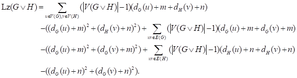
By the definition of join operation and the definition of Lanzhou index, we have following observation.
Observation 3. Let ![]() and
and ![]() are two graphs with
order
are two graphs with
order ![]() and
and ![]() , respectively. Then we have
, respectively. Then we have
Theorem 6.2. Let ![]() be a graph with order
be a graph with order ![]() and size
and size ![]() ,
and let H be a graph with order
,
and let H be a graph with order ![]() and size
and size ![]() .
Then we have
.
Then we have
![]() .
.
where ![]() .
.
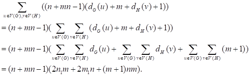
Proof. From Observation 16, we have that
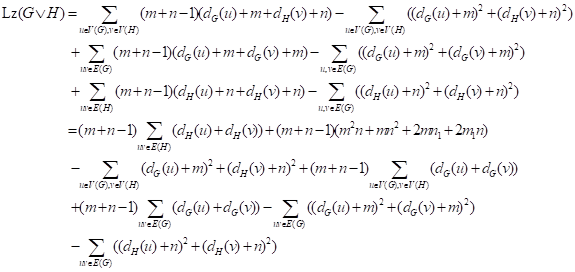
It is obviously, we have that
So, we have following equation.
![]()
Equation 1
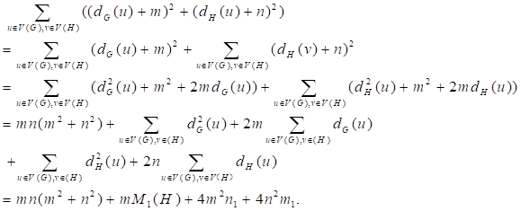
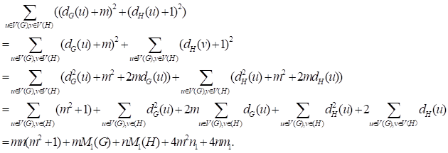
It is obviously that
So, we get equation
![]() Equation
2
Equation
2
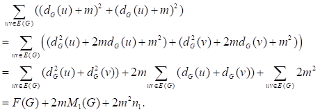
It is obviously that
So, we get equation
Equation 3
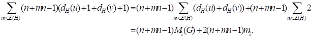
Similarly, we get equation
![]()
Equation 4
By equation Equation 1, Equation 2, Equation 3, and Equation 4, we have
![]() .
.
Where ![]() .
.
Let ![]() be a graph with order
be a graph with order ![]() .
The Corona of
.
The Corona of ![]() and
and ![]() is defined as the graph obtained by taking one
copy of graph
is defined as the graph obtained by taking one
copy of graph ![]() and taking n copy of graph
and taking n copy of graph ![]() ,
then, join ith vertex of
,
then, join ith vertex of ![]() to the vertexs in the i th copy of
to the vertexs in the i th copy of ![]() .
.
Observation 4. Let ![]() and
and ![]() be two graphs,
be two graphs,
![]() and
and ![]() .
Then we have
.
Then we have
By Observation 18, we have result as below.
Theorem 6.3. Let ![]() be a graph with order
be a graph with order ![]() and size
and size ![]() ,
and let
,
and let ![]() be a graph with order
be a graph with order ![]() and size
and size ![]() .
Then we have Let
.
Then we have Let
![]() .
.
where
![]() .
.
Proof. By Observation 18, it follows that
It obviously that
So, we have following equation
![]()
Equation 5
Since that
So, it follows that
![]()
Equation 6
Since that
![]()
So, it follows that
![]()
Equation 7
Since that
So, it follows that
![]()
Equation 8
So, it follows that
![]()
Equation 9
Since that
So, it follows that
![]()
Equation 10
By Equation 5, Equation 6, Equation 7, Equation 8, Equation 9, and Equation 10, we have that
![]() .
.
where ![]() .
.
CONFLICT OF INTERESTS
None.
ACKNOWLEDGMENTS
The third author was supported by the National Science Foundation of China (Nos. 11601254, 11551001, 11161037, 61763041, 11661068, and 11461054) and the Qinghai Key Laboratory of Internet of Things Project (2017-ZJ-Y21).
REFERENCES
Chartrand, G., Lesniak, L., and Zhang, P. (1996). Graphs and Digraphs. Chapman & Hall.
Furtula, B., and Gutman, I. (2015). A Forgotten Topological Index. Journal of Mathematical Chemistry, 53(4), 1184–1190. https://doi.org/10.1007/s10910-015-0480-z.
Hinz, A. M., and Schief, A. (1990). The Average Distance on the Sierpiński Gasket. Probability Theory and Related Fields, 87(1), 129–138. https://doi.org/10.1007/BF01217750.
Husimi, K. (1950). Note on Mayer’S Theory of Cluster Integrals. Journal of Chemical Physics, 18(5), 682–684. https://doi.org/10.1063/1.1747725.
Kaimanovich, V. A. (2001). Random Walks on Sierpiński Graphs : Hyperbolicity and Stochastic Hom-Ögbenization, Fractals in Graz, 145–183.
Kazemi, R., and Behtoei, A. (2017). The First Zagreb and Forgotten Topological Indices of D-Ary Trees, Hac-Ettepe. Journal of Mathematics and Statistics, 46(4), 603–611.
Klix, F., and Goede, K. R. (1967). Struktur and Komponenten analyse von Problem lö sungsprozersen. Zeitschrift für Psychologie, 174, 167–193.
Manuel, P., and Rajasingh, I. (2009). Topological Properties of Silicate Networks, IEEE.GC.Confe.Exhi, 5, 1–5. https://doi.org/10.1109/IEEEGCC.2009.5734286.
Nadeem, M. F., Zafar, S., and Zahid, Z. (2015). On Certain Topological Indices of the Line Graph of Subdivision Graphs. Applied Mathematics and Computation, 271, 790–794. https://doi.org/10.1016/j.amc.2015.09.061.
Pisanski, T., and Tucker, T. W. (2001). Growth in Repeated Truncations of Maps, Atti Sem. Mat. Fis. Univ. Modena, 49, 167–176.
Teguia, A. M., and Godbole, A. (2006). Sierpiński Gasket Graphs and Some of their Properties, Australasia-n. J. Combin, 35, 181–192. https://doi.org/10.48550/arXiv.math/0509259.
Vukičević, D., Li, Q., Sedlar, J., and Dǒslić, T. (2018). Lanzhou Index, MATCH Commun. Match. Computers and Chemistry, 80, 863–876.
Zmazek, B., and Zerovnik, J. (2003). Computing the Weighted Wiener and Szeged Number on Weighted Cactus Graphs in Linear Time. Croatica Chemica Acta, 76, 137–143.
Zmazek, B., and Zerovnik, J. (2005). Estimating the Trac on Weighted Cactus Networks in Linear Time, Ni-nth International Conference on Information Visualisation, 536–541.
 This work is licensed under a: Creative Commons Attribution 4.0 International License
© Granthaalayah 2014-2022. All Rights Reserved.