COMPARATIVE STUDY OF WHITE GAUSSIAN NOISE REDUCTION FOR DIFFERENT SIGNALS USING WAVELET

 

Parul Saxena ¹ , Vinay Saxena ²

 

¹ Assistant Professor, Department of Computer Science, Soban Singh Jeena University, Almora, 263601, Uttarakhand, India

² Professor, Department of Mathematics, Kisan Post Graduate College Bahraich, 271801, Uttar Pradesh, India

 

1. INTRODUCTION

There are many different types of noises in the environment. White Noise, which is purely random noise and is having an impulse autocorrelation function and a flat power spectrum, it theoretically contains all frequencies in equal power. Band limited White Noise, which is very much similar to the white noise but with a flat power spectrum and a limited bandwidth that usually covers the limited spectrum of the device or the signal of interest Singh and Garg (2014). Narrowband Noise which processes with a narrow bandwidth such as 50/60 Hz from the electricity supply. Coloured Noise, its spectrum has a non-flat shape. Impulsive Noise, which consists of short duration pulses of random amplitude, time of occurrence and duration. Transient noise pulses consist of relatively long duration noise pulses such as burst noise Wolfe et al. (2009).

CI can perform well up to 95% for profoundly deaf patients if there is no interference of external noise or background noise but this is not the practical situation as in reality there are so many factors which may cause to create noise in the input signal submitted to the speech processor. This performance of CI is reduced by 30 to 60 % with the interference of the external noise. With the studies it also has been proved that the children, who resides in noise most of the time, may perform well in comparison to the adults residing in noise Razza et al. (2017).

 

2. BASIC TERMINOLOGIES

2.1.  White Gaussian Noise

 Gaussianity refers to the probability distribution with respect to the value or the probability of the signal falling within any particular range of amplitudes. The term ‘white’ refers to the way the signal power is distributed independently over time or among frequencies Saxena and Mehta (2017).

 

2.2. Noise Cancellation

The existence of noise is inevitable in real applications of speech processing. In fact, background noise is one of the major factors that adversely affect the perceived grade of service in speech communication system. It is well known that the additive noise affects mainly the performance of the system and reduces the Signal to Noise Ratio (SNR) and the speech intelligibility. A noise reduction (NR) scheme, capable of handling a wide variety of noise situations with varying characteristics and noise levels, becomes necessary Saxena and Mehta (2017). The traditional approaches to noise cancellation lay in utilizing standalone noise cancellation modules on the near-side or transmit path. This approach works well under constant conditions, but as the environment changes, the performance gets degraded, and the system struggles to adapt Proakis and Manolakis (1996). The usual method of estimating a signal corrupted by additive noise is to pass it through a filter that tends to suppress the noise leaving the signal relatively unchanged i.e., direct filtering. The design of such filters is the domain of optimal filtering, which was originated with the pioneering work of Wiener and was extended by Kalman, Bucy and Others. Filters used for direct filtering can be either fixed or adaptive Saxena and Mehta (2017), Juang (1998), Lawrence (1978).

 

2.3. Wavelet for Noise Reduction

 Wavelet theory provides a unified framework for a number of techniques which had been developed independently for various signal processing applications. For example, multi resolution signal processing, used in computer vision; sub band coding, developed for speech and image compression; and wavelet series expansions, developed in applied mathematics, have been recently recognized as different views of a single theory Saxena and Mehta (2017), Misiti et al. (1996). In fact, wavelet theory covers quite a large area. It treats both the continuous and the discrete-time cases. It provides very general techniques that can be applied to many tasks in signal processing, and therefore has numerous potential applications Mallat (1999), Papoola (2006).  A wavelet is a waveform of effectively limited duration that has an average value of zero and nonzero norm. Sinusoidal waves are smooth and predictable, while wavelets tend to be irregular and asymmetric Saxena and Mehta (2017). Wavelet method is a basic method that is used for noise filtering, compression and analysis of non-stationary signals. It is an appropriate method for semi-stationary signals which provides a good resolution in both time and frequency domain. The wavelet transform produces better results than traditional methods in improving speech Gilbert (1996), Mark (1992).

 

2.4. Measures of Noise

 Here are some of the important terms to measure the noise parameters in the given signal.

 

2.4.1.  Signal To Noise Ratio

The signal-to-noise ratio (SNR) is commonly used to assess the effect of noise on a signal. The ratio between the power of signal and the power of noise defines the SNR Mark (1992). SNR is the ratio of signal power to the noise power. In terms of signals it indicates, how the original signal is affected by the added noise. SNR Saxena and Mehta (2017) is given by the following formula:

 

                          SNR= Average Signal Power / Average Noise Power

 

2.4.2.  Peak Signal to Noise Ratio

Peak signal¬ to noise ratio (PSNR) Saxena and Mehta (2017) is usually expressed in terms of the logarithmic decibel scale, where Max is the maximum value attained by the signal.

 

 

 

2.4.3.  Mean Absolute Error (MAE)

The MAE Saxena and Mehta (2017) measures the average magnitude of the errors I am set of forecasts, without considering their direction. It measures accuracy for continuous variables. The MAE is a linear score which means that all the individual differences are weighted equally in the average.

 

 

2.4.4.  Mean Squared Error (MSE)

The MSE Saxena and Mehta (2017) is a quadratic scoring rule. The difference between forecast and corresponding observed values are each squared and then averaged over the sample. This means the MSE is most useful when large errors are particularly undesirable.

 

3. NOISE REDUCTION ALGORITHM USING WAVELET

The noise is a stationary additive white Gaussian process, although for some problems this is a valid assumption and leads to mathematically convenient and useful solutions, in practice, the noise is often time varying, correlated, and non-Gaussian. This is particularly true for impulsive-type noise and for acoustic noise, which is non-stationary and non-Gaussian and hence cannot be modelled using the AWGN assumption.

In the Figure 1, whole mechanism for noise reduction process has been discussed. Initially the input signal is captured either by user or by input file then we add some noise in the signal. This noise is white in nature hence is uniformly distributed over the signal. The signal is decomposed in wavelet tree using wavelet packet decomposition process, then coefficients of wavelet tree are found. Alpha has been chosen 1.8, sigma and threshold are calculated. The resulting tree is refined by using these parameters and finally the denoised output is constructed. Here we have decomposed the signal into a wavelet tree of level 10 by using wpdec command. The coefficients of wavelet are determined by using wpcoef command. Here SIGMA is the standard deviation of the zero mean Gaussian white noise in the de-noising model. ALPHA is a tuning parameter Typically ALPHA = 2. THR = wpbmpen (T, SIGMA, ALPHA) returns a global threshold THR for de-noising. The speech of user is recorded by using wav record function in a file then this file is played by using wavplay function or sound function. Figure 2 shows one of the inputs captured by the end user.

 Figure 1

                                                                      

Figure 1 Flow Chart for Noise Reduction Process

 

Figure 2

                                                                     

Figure 2 Graphical Representation of Speech

 

Figure 3

                                                                     

Figure 3 Graphical user Interface for Noise Reduction

 

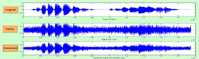
In the Figure 3, graphical user interface has been represented for noise reduction of input signal. This GUI has been designed using MATLAB. Original input signal is captured from the original button as represented in first window. Noise is added by using noisy button and noisy signal is represented in second window. Finally, by using denoised button the noisy signal is denoised and the denoised signal is shown in third window.

Here we have taken the inputs from different sound signals, and we have applied noise reduction algorithm using different types of wavelets. We have added white gaussian noise in these images and then finally we have reduced the noise by using above wavelet mechanism and we have found that the used mechanism is so efficient that we have received the results with very small error. We have shown the value of sigma, threshold, Mean Absolute Error, Mean Squared Error, Signal to Noise Ratio and Peak Signal to Noise Ratio in each case. These values have been represented in Table 1. The sampling frequency and the number of bits to represent a signal may vary. Here we have taken Sampling Frequency 22050 Hz. and Number of Bits 16.

Table 1

Table 1 Denoising of Signal1 “Bizarro.Wav” Using Different Types of Wavelets
Type of Wavelet	Sigma	Threshold	MAE	MSE	SNR	PSNR
Coif1	0.14095	0.449154	0.056216	0.005977	48.52663	55.954958
Coif2	0.090327	0.244157	0.038454	0.00271	51.961226	59.98354
Coif3	0.122716	0.378344	0.048435	0.004451	49.806417	57.460849
Coif4	0.10475	0.302829	0.042072	0.003323	51.075919	58.948969
Coif5	0.051066	0.096518	0.052083	0.004281	49.975906	57.659845
Db5	0.153445	0.488082	0.054482	0.005715	48.720778	56.183788
Db15	0.177622	0.596982	0.060972	0.007276	47.672551	54.946645
Db25	0.110033	0.322024	0.046252	0.004086	50.17802	57.897016
Db35	0.159884	0.539696	0.060144	0.007194	47.721505	55.004514
Db45	0.089805	0.229135	0.042206	0.003151	51.30736	59.219679
Sym5	0.08846	0.23058	0.039758	0.002797	51.825054	59.824575
Sym15	0.067	0.150847	0.039931	0.002616	52.115584	60.163662
Sym25	0.058268	0.131216	0.042658	0.002925	51.630523	59.597379
Bior1.1	0.139954	0.430141	0.062899	0.007351	47.627763	54.893692
Bior1.3	0.107955	0.292448	0.048977	0.004394	49.862874	57.527145
Bior1.5	0.119444	0.33824	0.049104	0.004524	49.736338	57.37854

 

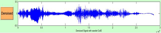
Original Signal1 “Bizarro.wav” and Noisy Signal1 “Bizarro.wav” are shown in Figure 4 and Figure 5 respectively. Various noise reduction mechanism using wavelet coiflet1, wavelet coiflet 2, wavelet coiflet 3, wavelet coiflet 4 and wavelet coiflet 5 are shown in Figure 6, Figure 7, Figure 8, Figure 9 and Figure 10 respectively. From these figures and Table 1, it is observed that the results obtained from wavelet Coif2 are the best for this noise reduction mechanism among all studied coiflet wavelets in Signal1 “Bizarro.wav”.

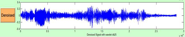
The Figure 11, Figure 12, Figure 13, Figure 14 and Figure 15 represents the noise reduction mechanism using wavelet Daubechies 5, wavelet Daubechies 15, wavelet Daubechies 25, wavelet Daubechies 35 and wavelet Daubechies 45 respectively. From these figures and Table 1, it is observed that the results obtained from wavelet Db45 are the best for this noise reduction mechanism among all studied Daubechies wavelets as it produces highest SNR and PSNR and least MSE, MAE in Signal1 “Bizarro.wav”.

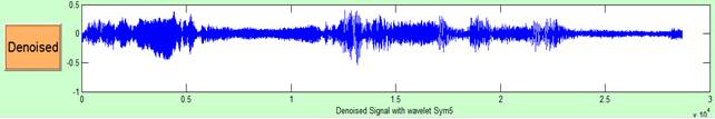
The Figure 16, Figure 17 and Figure 18 represents the noise reduction mechanism using wavelet Symlet 5, wavelet Symlet 15 and wavelet Symlet 25 respectively. From these figures and table 1, it is observed that Sym25 produces least MSE and highest SNR and PSNR while Sym15 produces least MAE for this noise reduction mechanism in Signal1 “Bizarro.wav”.

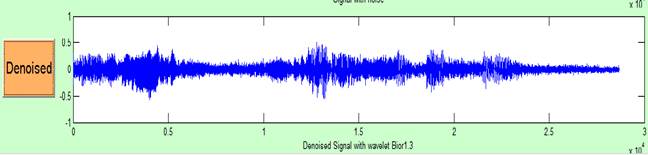
The Figure 19, Figure 20 and Figure 21 represents the noise reduction mechanism using wavelet Biorthogonal 1.1, wavelet Biorthogonal 1.3 and wavelet Biorthogonal 1.5 respectively. From these figures and table 1, it is observed that Bior1.3 produces the best results by producing least MAE, MSE and highest SNR and PSNR for this noise reduction mechanism in Signal1 “Bizarro.wav”.

Figure 4

                                                                       

Figure 4 Original Signal1 “Bizarro.wav”

Figure 5

                                                                     

Figure 5 Noisy Signal1 “Bizarro.wav”

 

Figure 6   

                                                                       

Figure 6 Signal1 “Bizarro.wav” Denoising using Wavelet Coiflet 1

 

Figure 7

                                                                       

Figure 7 Signal1 “Bizarro.wav” Denoising using Wavelet Coiflet 2

 

Figure 8

                                                                     

Figure 8 Signal1 “Bizarro.wav” Denoising using Wavelet Coiflet 3

 

Figure 9   

                                                                      

Figure 9 Signal1 “Bizarro.wav” Denoising using Wavelet Coiflet 4

 

Figure 10

                                                                     

Figure 10 Signal1 “Bizarro.wav” Denoising using Wavelet Coiflet 5

 

Figure 11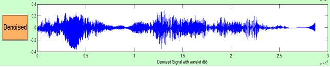

Figure 11 Signal1 “Bizarro.wav” Denoising using Wavelet Daubechies 5

 

Figure 12

                                                                     

Figure 12 Signal1 “Bizarro.wav” Denoising using Wavelet Daubechies 15

 

Figure 13

                                                                      

Figure 13 Signal1 “Bizarro.wav” Denoising using Wavelet Daubechies 25

 

Figure 14

                                                                     

Figure 14 Signal1 “Bizarro.wav” Denoising using Wavelet Daubechies 35

 

Figure 15

                                                                     

Figure 15 Signal1 “Bizarro.wav” Denoising using Wavelet Daubechies 45

 

Figure 16

                                                                     

Figure 16 Signal1 “Bizarro.wav” Denoising using Wavelet Symlet 5

 

Figure 17

                                                                     

Figure 17 Signal1 “Bizarro.wav” Denoising using Wavelet Symlet 15

 

Figure 18

                                                                     

Figure 18 Signal1 “Bizarro.wav” Denoising using Wavelet Symlet 25

 

Figure 19

                                                                     

Figure 19 Signal1 “Bizarro.wav” Denoising using Wavelet Biorthogonal 1.1

 

Figure 20

                                                                     

Figure 20 Signal1 “Bizarro.wav” Denoising using Wavelet Biorthogonal 1.3

 

Figure 21

                                                                      

Figure 21 Signal1 “Bizarro.wav” Denoising using Wavelet Biorthogonal 1.5

 

4. RESULT AND DISCUSSION

After analysing all the denoising Figure 6, Figure 7, Figure 8, Figure 9,Figure 10,

Figure 11, Figure 12, Figure 13, Figure 14, Figure 15, Figure 16, Figure 17, Figure 18, Figure 19, Figure 20, Figure 21 and Table 1, we observed the concluding Table 2 which suggests the best results are obtained using wavelet coiflet 2 for Signal1 “Bizarro.wav”. Table 2 represents the values of sigma, threshold, MAE, MSE SNR and PSNR for the signal bird.wav. The noise reduction mechanism has been applied for this signal under various categories of wavelets. Here the produced sampling frequency Fs is 22050 Hz. and number of bits n bits used for coding are 16. As we have found that the developed algorithm for noise reduction is working efficiently with wavelet coiflet2, so we are applying this algorithm on different types of signals using wavelet coiflet2. The input signals may or may not contain noise. The Gaussian noise is added than the noise reduction algorithm is applied. The inputs taken here cover a very large domain and contain the sounds of various amplitude and frequencies. Mainly these inputs cover the sounds from various species as dog, dove, bizarro, pig, frog etc, sounds from vehicles as train, helicopter etc, sounds of chimes, bubbles etc. Then we have applied the developed algorithm on these sounds of varying domain.

Table 2

Table 2 Results for Noise Reduction Mechanism for Signal1 “Bizarro.Wav”
Attribute Name	Lowest	Highest
Sigma	Coif2	DB35
Threshold	Coif2	DB35
MAE	Coif2	Bior1.1
MSE	Coif2	Bior1.1
SNR	Bior1.1	Coif2
PSNR	Bior1.1	Coif2

 

5. CONCLUSION

It is observed that the developed algorithm for noise reduction using wavelet works very well for different types of wavelets. Although it gives good results for all kinds of wavelets, it performs the best using wavelet coiflet 2. The successful implementation of this denoising algorithm for different types of inputs, lying in different domains, makes it versatile. Finally, we have implemented the algorithm on different levels of input SNR, and we have found that as soon as the SNR increases the PSNR is also increased and simultaneously MAE and MSE are decreased, and a higher value of SNR gives the best results.

 

CONFLICT OF INTERESTS

None. 

 

ACKNOWLEDGMENTS

None.

 

REFERENCES

Gilbert, S., (1996). Wavelets And Filter Banks, Wellesley Cambridge Press,1-34.

Juang, B.H., (1998). The Past Present and Future of Speech Processing, IEEE Signal Processing Magazine, 15(3), 24-48. https://doi.org/10.1109/79.671130

Lawrence, R. R., (1978). Digital Processing of Speech Signals, Englewood Cliffs New Jersey : Prentice Hall Inc,43-55, 130-135.

Mallat, S., (1999). A Wavelet Tour of Signal Processing, Second Edition, Academic Press. New York.

Mark, J. S., (1992). The Discrete Wavelet Transform : Wedding A Tours and Mallat Algorithms, IEEE Transactions on Signal Processing,40(10),2464-2482. https://www.doi.org/10.1109/78.157290

Misiti, M., Misiti, Y., Oppenheim, G., and Poggi, J. M., (1996). Wavelet Toolbox User’s Guide Computation, The Math Works, Inc.,1-1030.

Papoola, A., (2006). Testing the Suitability of Wavelet Preprocessing for TSK Fuzzy Models, IEEE International Conference on Fuzzy Systems Sheraton Vancouver Wall Centre Hotel, Vancouver, BC, Canada, 16-21. https://doi.org/10.1109/FUZZY.2006.1681878

Proakis, J.G., Manolakis, D.G., (1996). Digital Signal Processing Principles, Algorithms, Third Edition, Prentice Hall International Inc., New Jursy,1-1033.

Razza, S., Zaccone, M., Meli, A., and Cristofari, E., (2017). Evaluation of Speech Reception Threshold in Noise in Young Cochlear Nucleus System 6 Implant Recipients using Two Different Digital Remote Microphone Technologies and A Speech Enhancement Sound Processing Algorithm, International Journal of Pediatric Otorhinolaryngology, Elsevier 103,71–75. https://doi.org/10.1016/j.ijporl.2017.10.002

Saxena, P., Mehta, A., (2017).  Study of White Gaussian Noise With Varying Signal To Noise Ratio in Speech Signal using Wavelet, American International Journal of Research in Science, Technology, Engineering and Mathematics ,19(1), 133-137.

Singh, M., Garg, N. K. (2014). Audio Noise Reduction using Butter Worth Filter, International Journal of Computer and Organization Trends, 6(1) ,20-23.

Wolfe, J., Schafer, E. C., Heldner, B., Mulder, H., Ward, E., and Vincent, B. (2009). Evaluation of Speech Recognition in Noise with Cochlear Implants and Dynamic FM, J Am Acad Audial 20,409-421. https://doi.org/10.3766/jaaa.20.7.3