DEVELOPING A MULTI-ITEM, MULTI-PRODUCT, AND MULTI-PERIOD SUPPLY CHAIN NETWORK DESIGN AND PLANNING MODEL FOR PERISHABLE PRODUCTS

1. INTRODUCTION

A supply chain (SC) is a complex network of activities, workers, technology and physical infrastructures, and policies involved in the procurement of raw materials, their transformation into products, and their logistics operations Hassan (2006). And supply chain management (SCM), according to Bank et al. (2020), is a process that tries to efficiently integrate the various phases of the supply chain to provide the right number of products to end-users at the right time. A framework for supply chain integration was developed by Huo et al. (2009). With globalization and the escalation of competition, effective supply chain design has become one of the most pressing concerns facing businesses, affecting all actions to create, improve quality, reduce costs, and provide services Hendalianpour et al. (2019).

At many decision levels, such as strategic, tactical, and operational, an efficient supply chain integration necessitates multiple coordinated decisions on items, information flow, and financial resources Farias et al. (2017). The variety and heterogeneity of stakeholders, many of whom have competing goals, make supply chain design and management extremely difficult Diabat et al. (2016), Hammami et al. (2017). Organizations always try to work together to achieve common goals on this problem Simchi-Levi et al. (2003).

Companies all around the world are competing not just on pricing and product quality, but also on delivery reliability because of growing globalization Guido et al. (2020). As a result, SCM research has exploded in recent years, with a particular focus on the integrated planning of production, storage, and distribution activities Viergutz and Knust (2014).

A good can be termed perishable, according to Amorim et al. (2013), if at least one of the following requirements occurs throughout a well-defined planning horizon: (1) its physical condition deteriorates, (2) it’s worth decreases, and (3) there is a possibility of future reduced functionality, as determined by some authority.

When the unique qualities of perishable products are taken into account, the SCM challenge becomes more difficult and demanding Chintapalli (2015). Perishable product inventory challenges have been extensively discussed in the earlier literature. The design of the perishable product supply chain network is rarely considered Tsao et al. (2021).

Perishable products are extremely important in a variety of industries, from food and pharmaceuticals to high-tech. According to Zahiri et al. (2014), the quality or quantity deteriorates over time and their value or functioning decreases, which can have unintended consequences.

The perishable nature of the organ influences kidney or heart transplants Zahiri et al. (2014), the chemical composition of medicines determines the period within which they are still effective Chung and Kwon (2016), and proper blood bank management is critical for patient health in hospitals Zahiri et al. (2014), Najafi et al. (2017).

Table 1

Table 1 Research on SSCND documents for perishable products.

Author

Objective Functions

Application

Multi-item

Multi-product

Multi -period

Multi-customer

Single

Multi

Economic

Environmental

Social

Other

Dwivedi et al. (2020)

agro-food

Jiang et al. (2019)

beverage

Rohmer et al. (2018)

food

Eskandari-khanghahi et al. (2017)

blood

Patidar et al. (2019)

agro-food

Moghaddam et al. (2019)

meat

Varsei and Polyakovskiy (2015)

wine

Zahiri et al. (2017)

pharmaceutical

Al-Ashhab et al. (2021)

General

Our

General

As shown in Table 1, some research publications are addressing Sustainable Supply Chain Network Design (SSCND) for perishable products. So, the purpose of this research is to solve the problem of design and planning supply chain of multi-item perishable products. A mathematical model for designing a multi-period, four-tiered supply network, including supplier, factory, distributor, and customer, has been developed using mixed integer nonlinear programming (MINLP).

2. PROBLEM DESCRIPTION

The goal of this model is to determine the optimal supply chain design and determine the optimal number of units to be produced in each period, the quantities of items to be transferred from suppliers to factories, from factories to the distributor and from the distributor to customers considering perishability of the product, the demand of the customer, and the management of the inventory according to the ages of products in the inventory. The model also aids in reducing product waste and expiration, avoiding increased costs and pollution from additional transportation.

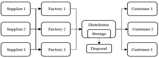
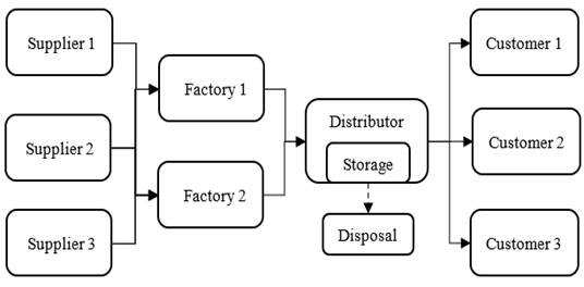
This multi-item, multi-product perishable model has been developed based on the model proposed by Al-Ashhab et al. (2021). The supply chain network has been extended to include three potential uppliers, three potential factories, one distributor, and three customers as shown in Figure 1

Figure 1

Figure 1 The proposed supply chain network

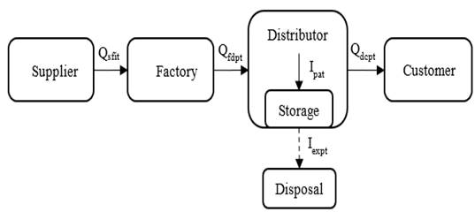
The relationship between the different facilities is shown in Figure 2

Figure 2

Figure 2 Model flow

3. MODEL ASSUMPTIONS AND FORMULATION

The mathematical model is built on the following assumptions.

· The demands of customers are known and deterministic.

· Each product consists of multiple items.

· Products have a known and limited shelf life.

· The first products produced are issued first.

· There is no initial inventory.

· Expired products are treated as waste and discarded.

· The capacities of all facilities are known and limited.

· The backlog is allowed.

The model involves the following sets, parameters, and decision variables:

Sets:

· S, F, D, and C: possible locations of suppliers, factories, distributors, and customers.

· I: number of items (indexed by i = 1...I).

· P: number of products.

· A: ages of products.

· T: number of periods.

Parameters

· DEMANDcpt: Demand of customer c of product p in period t.

· SL: Shelf-life duration of product p after the finish of its production.

· CAPsit: Capacity of supplier s for item i in period t.

· CAPMft: Capacity of the factory raw material stock up in period t.

· CAPHft: Capacity in production hours of the factory f in period t.

· CAPdt: Distributor capacity r in period t.

· MATCOSTsit: Material cost per unit of item i supplied by supplier s in period t.

· MCft: Manufacturing cost per hour for factory f in period t.

· MHp: Manufacturing hours of the product (p).

· TC: Transportation cost per unit per kilometer.

· Dsf: Distance of supplier s to factory f.

· Dfd: Distance from factory f to distributor d.

· Ddc: Distance of distributor d to the customer c.

· TC: Transportation cost per unit per kilometer.

· Fs: Fixed cost of ordering for supplier s in period t.

· Ff: Fixed cost of the factory f.

· Fd: Fixed cost of the distributor d.

· Wi: Weight of item i (kg).

· REQip: Required quantity of item i for product p (unit).

· Wp: Weight of product p (kg).

· Ppt: Unit price of product p in period t ($).

· ECp: Expired cost per unit.

· SCp: Shortage cost per unit.

· IHCp: Cost of inventory maintenance per unit per period.

· NUCCF: Cost of non-utilized manufacturing capacity per hour of the factory.

· Bsi: Batch size of item i transferred from supplier s to factory f (unit).

· Bfp: Batch size transferred from the factory f for product p to the distributor d (unit).

· Bdp: Batch size transferred from the distributor d for product p to the customer c (unit).

Decision Variables

· Qsfit: Number of batches of items i transfer from suppliers s to factory f in period t.

· Qfdpt: Number of batches of product p transferred from factory f to distributor d in period t.

· Qdcpt: Number of batches transferred from factory f to customer c for product p in period t.

· Ipat: Number of batches transferred from factory f to its storehouse for the product p in period t.

· Iexpt: Stock expired at the end of period (t)

· Ls: Binary variable, equals 1 if supplier (s) is established; 0 otherwise.

· Lf: Binary variable, equals 1 if factory (f) is established; 0 otherwise.

· Z: total profit.

3.1. OBJECTIVE FUNCTION

The objective of the model is to maximize the profit of the supply chain. The profit is calculated by subtracting the total cost from the total revenue. The total revenue is calculated by using Equation 1

Equation 1

Total cost = fixed costs + material costs + manufacturing costs + non-utilized capacity costs + shortage costs + transportation costs + inventory holding costs + expired costs.

The costs appear Equation 2, Equation 14 as follows:

Equation 2

Equation 3

Equation 4

Equation 5

Equation 6

Equation 7

Equation 8

Equation 9

3.2. CONSTRAINTS

Equation 10

Equation 10 ensures that all suppliers are given within their limited capacities.

Equation 11

Equation 11 guarantees that the sum of the material flow that enters the factory from all suppliers does not exceed the material capacity of the factory in each period.

Equation 12

Equation 12 guarantees that the sum of manufacturing hours for all products manufactured in the factory to be delivered to each distributor does not override its manufacturing capacity hours in each period.

Equation 13

Equation 13 guarantees that the amount of materials entering the factories from all suppliers equals the sum of the exiting from it to each distributor.

Equation 14

Equation 14 ensure that, in the first period, the number of units transported from the factory to the distributor cannot override the distributor capacity.

Equation 15

Equation 15 ensures that the overall quantity of products from all the factories entering the distributor in each period and products residual from the previous period cannot override the distributor capacity.

Equation 16

Equation 16 guarantees that in the first period, the sum of the flow entering each customer cannot override the sum of the existing period demand.

Equation 17

Equation 17 guarantees that the sum of the flowing entering each customer does not override the sum of the present period demand and the former cumulative shortages for each product.

Equation 18

Equation 18 ensures that before the shelf-life period is reached there can be no expired stock.

Equation 19

Equation 19 ensures that expired inventory appears only after the shelf life is reached.

Equation 20

Equation 20 ensures that inventory of all ages in all periods cannot have a negative value.

Equation 21

Equation 21 ensures that the inventory is equal to zero when the age is greater than the period.

Equation 22

Equation 23

Equation 24

Equation 22, Equation 23, and Equation 24 ensure that the demand is fulfilled first through the stock of the oldest age products in the distributor's inventory, and then the stock of the next in age until we reach the stock of the youngest age.

4. RESULT AND ANALYSIS

The model is solved using GAMS software and ran on an Intel ® Core™ i5-1035G7 CPU @ 1.50 GHz (8 GB of RAM). Through the following study, the model parameters were considered as shown in Table 2.

Table 2

Table 2 The parameters assumed for model verification in the case study
No.	Input parameter	Value	Unit	No.2	Input parameter3	Value4	Unit5
1	S and F	3	–	19	MATCOSTit 1,2	1, 2, 3	$/kg
2	D	1	–
3	C	3	–	20	MHp 1,2	1, 2	Hrs
4	I	2	–	21	MCft 1,2,3	10	$/hr
5	P	2	–	22	SL	3	hrs
6	A	3	–	23	TC	0.002	$/Km
7	T	6	–	24	Ds1f	5, 8, 12	Km
8	Fs and Ff	10000,15000 ,20000	$	25	Ds2f	13, 17, 22	Km
9	Fd	10000	$	26	Ds3f	17, 20, 25	Km
10	Wi 1,2	1	Kg	27	Dfd	100, 150, 200	Km
11	Wp 1,2	3, 6	Kg	28	Ddc	100,150, 200	Km
12	REQip 1	1, 2	Kg. /Unit	29	Bsi	1	Unit
13	REQip 2	2, 4	Kg. /Unit	30	Bfp	1	Unit
14	Ppt	100, 150	$/Unit	31	Bdp	1	Unit
15	ECp 1,2	1, 2	$/Unit	32	CAPSit 1,2	3000	Kg
16	SCp 1,2	5, 10	$/period	33	CAPMft 1,2,3	6000	Kg
17	IHCp 1,2	1, 1	$/kg. period	34	CAPHft 1,2,3	6000	Hrs
18	NUCCF	3	$/hr	35	CAPdt	60000	unit

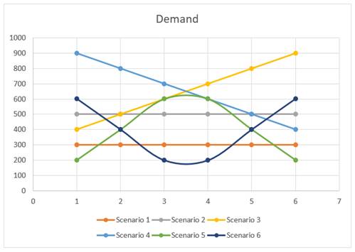
Six scenarios have been conducted with different demands as shown in Table 3 and Figure 3 to study and analyse the effect of the demand pattern on the supply chain.

Table 3

Table 3 Demand for each customer from each product in each period in the six scenarios
Period	T₁	T₂	T₃	T₄	T₅	T₆
Scenario 1	300	300	300	300	300	300
Scenario 2	500	500	500	500	500	500
Scenario 3	400	500	600	700	800	900
Scenario 4	900	800	700	600	500	400
Scenario 5	200	400	600	600	400	200
Scenario 6	600	400	200	200	400	600

Figure 3

Figure 3 Demand patterns for each customer from each product in each period in the six scenarios

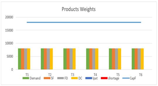
4.1. SCENARIO 1

The optimal supply chain network for the first scenario is shown in Figure 4. As shown in Figure 5, it is observed that the total required weights of 8100 kg for all periods are less than the manufacturing capacity in all periods, so the factory satisfied all demands without any shortage.

Figure 4

Figure 4 Optimal supply chain network of the first scenario

Figure 5

Figure 5 Product weights

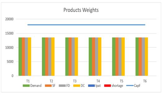
4.2. SCENARIO 2

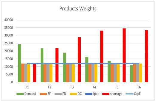
The optimal supply chain network for the second scenario is as shown in Figure 1. In Figure 6, it is noticed that the required weights for all periods of 13500 kg are less than the manufacturing capacity in all periods, so the factory satisfied all demands without any shortage.

Figure 6

Figure 6 Product Weights

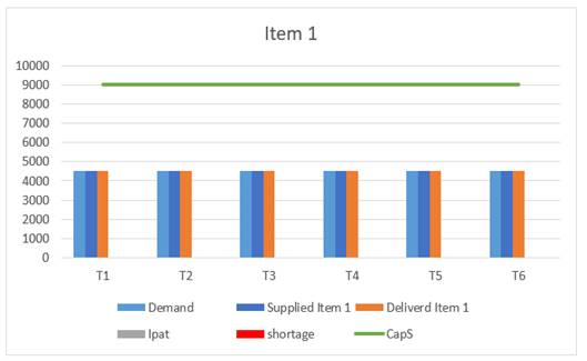
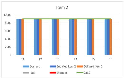
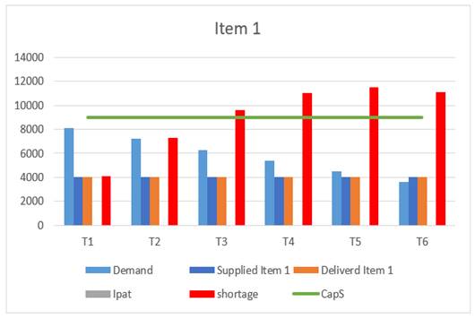
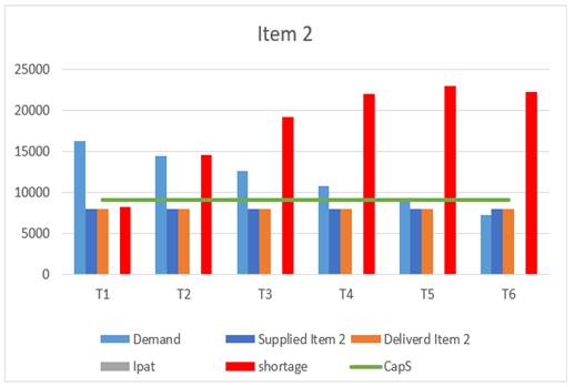
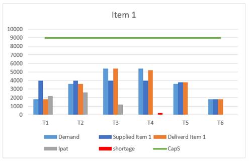
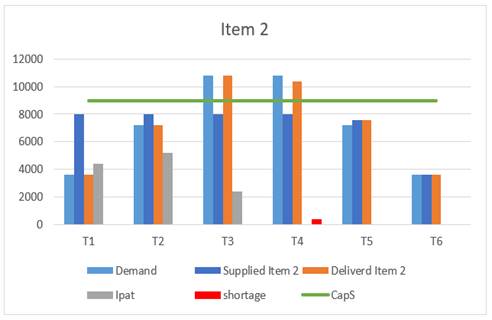
Figure 8 and Figure 9 show the relation between the demand and delivered quantities of the first and second item and the inventory, shortage, and the supplier capacity. As shown in Figure 8, it is noticed that the required weight of the second item, 4500 Kg, is less than the suppliers' capacities. In all periods, the suppliers can satisfy all demands without shortages. While as shown in Figure 9, it is noticed that the required weight of the second item, 9000 kg, is equal to the suppliers' capacities of the suppliers (3 * 3000 = 9000 kg). In all periods, the suppliers can just satisfy all demands without shortages.

Figure 7

Figure 7 the relation between the demand and delivered quantities of the first item

Figure 8

Figure 8 the relation between the demand and delivered quantities of the second item

4.3. SCENARIO 3

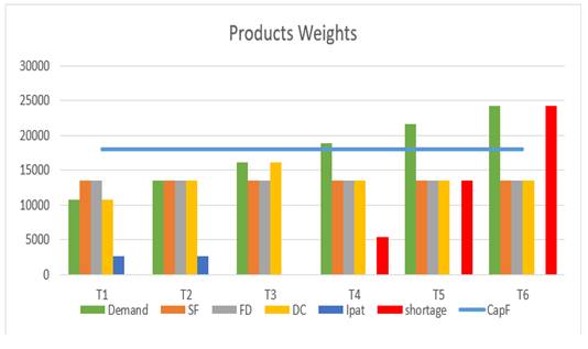
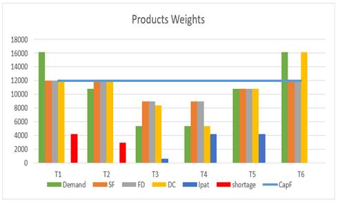
The optimal supply chain network for the third scenario is as shown in Figure 1. As shown in Figure 9, it is noted that the required weights are 10800, 13500, 16200, 18900, 21600, and 24300 kg. The required weight in the first, second, and third periods is less than the capacity of the factories, and in the fourth, fifth, and sixth periods the required weight exceeds the capacity of the factories, so production was carried out with the full capacity of the factories in all periods and the excess amount of the required weight was stored in the first two periods to reduce the expected shortage in the later periods.

Figure 9

Figure 9 Products Weights

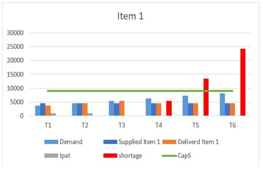
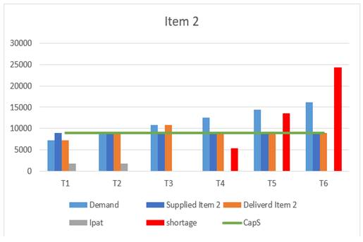
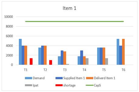
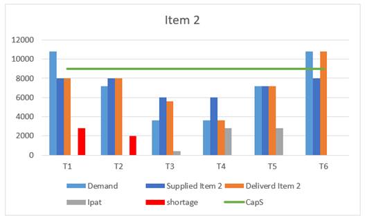
As shown in Figure 10 and Figure 11, it is noticed that in periods 1, the delivered weights were more than required. The excess quantity was stored in the first two periods to meet the high demand in the third period. In period 3, the suppliers delivered their full capacity from item 2 as shown in Figure 11. In periods 4, 5, and 6, the required weights from item 2 are more than the suppliers' capacities so the factories cannot satisfy all demands and there will be a shortage in these three periods.

Figure 10

Figure 10 the relation between the demand and the quantities delivered of the first item

Figure 11

Figure 11 the relation between the demand and the quantities delivered for the second item

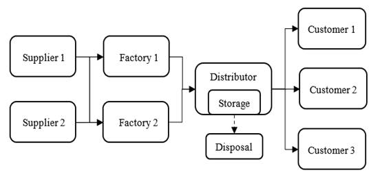
4.4. SCENARIO 4

Figure 12

Figure 12 supply chain network for the fourth scenario

Figure 12 shows the optimal supply chain network for the fourth scenario. As shown in Figure 13, it is noted that the required weights are 24300, 21600, 18900, 16200, 13500, and 10800 kg. In periods 1, 2, 3, 4, and 5, the required weights are more than those delivered in the same period, which is limited by the factory raw material store of 3,000 kg for each factory, and only two factories were operated, for a total of 12,000 kg. Therefore, the factories are not able to meet the demands of the customers and there will be some shortages. In 6 periods, the weights delivered were more than required in the same period to reduce some of the shortage occurred in the previous periods.

Figure 13

Chart, bar chart

Description automatically generated

Figure 13 Products Weights

As shown in Figure 14 and Figure 15, in 1, 2, 3, and 4 periods, the required weight is more than the factories' material capacities because the model only opens 2 factories, which means they can take only 12000 kg from all suppliers. It is equal in period 5 and less than in period 6. Factories cannot satisfy all demands and there will be a shortage.

Figure 14

Figure 14 the relation between the demand and the quantities delivered of the first item

Figure 15

Figure 15 the relation between the demand and the quantity delivered of the second item

4.5. SCENARIO 5

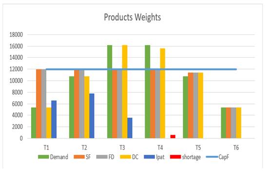
Figure 12 shows the optimal supply chain network for the fifth scenario. As shown in Figure 16, it is observed that the required weights are 5400, 10800 16200, 16200, 10800, and 5400 kg. The model decided to open only two factories. In periods 1 and 2, the delivered weights were more than those required in the same periods. The excess quantities were stored in the first two periods to meet the high demand in the third and fourth periods.

In periods 3 and 4, the factories delivered 16,200 and 15,600 kg using their full capacity and the remaining inventory from the previous period. But there is some shortage in the fourth period because the factories and the remaining stocks are unable to meet the high demand. To satisfy the shortage in the fourth period, the delivered weights are more than those required in the same period in period 5. In period 6, the required weights were less than the manufacturing capacity, so the factories met the demand without any shortage.

Figure 16

Figure 16 Products Weights

As shown in Figure 17 and Figure 18, it is noticed that in periods 1 and 2, the delivered weights were higher than those required in the same period for period 1 and equal in period 2. The excess quantity of required weight was stored in the first two periods to meet the high demand in the later periods.

In periods 3, and 4, the suppliers delivered items that were limited by the material capacity of factories and inventory remaining from the previous period. But there is a shortage in the fourth period because the suppliers and the remaining stocks are unable to meet the high demand.

To satisfy the shortage in the fourth period, in period 5, the delivered items are more than those required in the same period. In period 6, the required items were less than the materials capacity for factories, so the suppliers satisfied demand without any shortage.

Figure 17

Figure 17 the relation between the demand and the quantities delivered of the first item

Figure 18

Figure 18 the relation between the demand and delivered quantities of the second item

4.6. SCENARIO 6

Figure 12 shows the optimal supply chain network for the sixth scenario. As shown in Figure 19, it is noted that the required weights are 16200, 10800, 5400, 5400, 10800, and 16200 kg.. The model decided to open only two factories. In period 1, the required weights are more than those delivered in the same period, which is limited by the factory raw material store of 3,000 kg for each factory, and only two factories were operated, for a total of 12,000 kg. Therefore, the factories are not able to meet the demands of the customers and there will be some shortages.

In periods 2, 3, and 4, the weights delivered were more than required in the same period to satisfy the shortage in the first period and to satisfy high demand in the sixth period. In period 5, the required weights were less than the manufacturing capacity, so the factories satisfied demand, and they stored 4,200 to cover the high demand in the sixth period. In period 6, the factories delivered 16,200 kg using their full capacity and the inventory remaining from the previous period.

Figure 19

Figure 19 Product Weights

As shown in Figure 20 and Figure 21, it is observed that in period 1, the required items are more than those delivered in the same period, which means that the suppliers cannot meet the demand due to the capacity of the materials factories because the model has only opened two factories, a total of 12,000 kg, and there will be some shortages.

In periods 2, 3, and 4, the items delivered were more than required in the same period to satisfy the shortage in the first and second periods and to satisfy the high demand in the sixth period.

In period 5, the required items were less than the suppliers' capacity, so the suppliers satisfied demand, and they stored the remaining items to cover the high demand in the sixth period. While in period 6, the suppliers delivered items using their full capacity and the remaining inventory from the previous period.

Figure 20

Figure 20 the relationship between the demand and delivered quantities of the first item

Figure 21

Figure 21 the relationship between the demand and the quantities delivered for the second item

5. CONCLUSION AND FUTURE DEVELOPMENTS

In this paper, a sustainable supply chain network design model for multi-item, multi-perishable products was presented to prevent product expiry using the FIFO inventory strategy in order to maximize the network's total profit while minimizing environmental impact by reducing expiration waste.

The model effectively handled the problem of designing a long-term supply chain network for multi-item, multi-perishable products that take into account multi-period inventory in the storehouse as well as backlog, where unfulfilled demand in one period can be met in succeeding periods. It has aided in the prevention of product expiration by ensuring that only the needed quantities are produced with no waste.

Different scenarios were used to verify the model's results. The avoidance of product expiration resulted in maximizing profits while reducing environmental effects.

It is proposed that the model be developed to the following:

· Optimize multi-objectives, such as maximizing overall service level and minimizing total cost.

· Deal with the problem of stochastic demand.

· Considering robustness.

REFERENCES

Al-Ashhab, M. S. Nabil, O. M. And Afia, N. H. (2021). Perishable products supply chain network design with sustainability, Indian J. Sci. Technol., 14(9), 787-800. https://doi.org/10.17485/IJST/v14i9.24

Amorim, P. Meyr, H. Almeder, C. And Almada-Lobo, B. (2013). Managing perishability in production-distribution planning : A discussion and review, Flex. Serv. 25(3), 389-413. https://doi.org/10.1007/s10696-011-9122-3

Bank, M. Mazdeh, M. M. And Heydari, M. (2020). Applying meta-heuristic algorithms for an integrated production-distribution problem in a two level supply chain, Uncertain Supply Chain Manag., 8(1), 77-92. https://doi.org/10.5267/j.uscm.2019.8.004

Biuki, M. Kazemi, A. And Alinezhad, A. (2020). An integrated location-routing-inventory model for sustainable design of a perishable products supply chain network. https://doi.org/10.1016/j.jclepro.2020.120842

Chintapalli, P. (2015). Simultaneous pricing and inventory management of deteriorating perishable products, 229(1), 287-301. https://doi.org/10.1007/s10479-014-1753-9

Chung, S. H. And Kwon, C. (2016). Integrated supply chain management for perishable products : Dynamics and oligopolistic competition perspectives with application to pharmaceuticals, 117-129. https://doi.org/10.1016/j.ijpe.2016.05.021

Diabat, A. Abdallah, T. And le, T. (2016). A hybrid tabu search based heuristic for the periodic distribution inventory problem with perishable goods, Ann. Oper. Res., 242(2), 373-398. https://doi.org/10.1007/s10479-014-1640-4

Dwivedi, A. Jha, A. Prajapati, A. Sreenu, N. and Pratap, S. (2020). Meta-heuristic algorithms for solving the sustainable agro-food grain supply chain network design problem, Mod. Supply Chain Res. Appl., 2(3), 161-177. https://doi.org/10.1108/MSCRA-04-2020-0007

Eskandari-khanghahi, M. Tavakkoli-moghaddam, R. Taleizadeha, A. A. and Amind, S. H. (2017). Engineering Applications of Artificial Intelligence Designing and optimizing a sustainable supply chain network for a blood platelet bank under uncertainty, 236-250. https://doi.org/10.1016/j.engappai.2018.03.004

Farias, E. D. S. Li, Q. J. Galvez, L. P. And Borenstein, D. (2017). Simple heuristic for the strategic supply chain design of large-scale networks : A Brazilian case study, Comput. 746-756. https://doi.org/10.1016/j.cie.2017.07.017

Guido, R. Mirabelli, G. Palermo, E. And Solina, V. (2020). A framework for food traceability : Case study-Italian extra-virgin olive oil supply chain, 11(1), 50-60. https://doi.org/10.24867/IJIEM-2020-1-252

Hammami, R. Frein, Y. And Bahli, B. (2017). Supply chain design to guarantee quoted lead time and inventory replenishment: model and insights, 55(12), 3431-3450. https://doi.org/10.1080/00207543.2016.1242799

Hassan, M. M. D. (2006). Engineering supply chains as systems, Syst. Eng., 9(1), 73-89. https://doi.org/10.1002/sys.20042

Hendalianpour, A. et al. (2019). Hybrid Model of IVFRN-BWM and Robust Goal Programming in Agile and Flexible Supply Chain, a Case Study: Automobile Industry, IEEE Access, 7,71481-71492. https://doi.org/10.1109/ACCESS.2019.2915309

Huo, Y. Jiang, X. Jia, F. And Li, B. (2009). A Framework and Key Techniques for Supply Chain Integration, Supply Chain W. to Flat Organ. https://doi.org/10.5772/6661

Jiang, Y. Zhao, Y. Dong, M. And Han, S. (2019). Sustainable Supply Chain Network Design with Carbon Footprint Consideration : A Case Study in China, Math. Probl. https://doi.org/10.1155/2019/3162471

Moghaddam, S. T. Javadi, M. And Molana, S. M. H. (2019). A reverse logistics chain mathematical model for a sustainable production system of perishable goods based on demand optimization, 15(4), 709-721. https://doi.org/10.1007/s40092-018-0287-1

Najafi, M. Ahmadi, A. And Zolfagharinia, H. (2017). Blood inventory management in hospitals : Considering supply and demand uncertainty and blood transshipment possibility, Oper. 43-56. https://doi.org/10.1016/j.orhc.2017.08.006

Patidar, E. Venkatesh, B. Pratap, S. And Daultani, Y. (2019). A Sustainable Vehicle Routing Problem for Indian Agri-Food Supply Chain Network Design. https://doi.org/10.1109/POMS.2018.8629450

Rohmer, S. U. K. Gerdessen, J. C. And Claassen, G. D. H. (2018). Sustainable supply chain design in the food system with dietary considerations : A multi-objective analysis. https://doi.org/10.1016/j.ejor.2018.09.006

Simchi-Levi, D. Wu, S. D. and Shen, Z. M. (2003). Designing and Managing Supply Chain. https://doi.org/10.1007/978-1-4020-7953-5_1

Tsao, Y.C. Zhang, Q. Zhang, X. And Vu, T. L. (2021). Supply chain network design for perishable products under trade credit, 38(6), 466-474. https://doi.org/10.1080/21681015.2021.1937722

Varsei, M. And Polyakovskiy, S. (2015). Sustainable supply chain network design : A case of the wine industry in Australia Reference. https://doi.org/10.1016/j.omega.2015.11.009

Viergutz, C. and Knust, S. (2014). Integrated production and distribution scheduling with lifespan constraints, Ann. Oper. Res., 213(1),293-318. https://doi.org/10.1007/s10479-012-1197-z

Zahiri, B. Tavakkoli-Moghaddam, R. and Pishvaee, M. S. (2014). A robust possibilistic programming approach to multi-period location-allocation of organ transplant centers under uncertainty, Comput. 74(1), 139-148. https://doi.org/10.1016/j.cie.2014.05.008

Zahiri, B. Zhuang, J. and Mohammadi, M. (2017). Toward an integrated sustainable-resilient supply chain : A pharmaceutical case study, Transp. Res. Part E, 103, 109-142. https://doi.org/10.1016/j.tre.2017.04.009

This work is licensed under a: Creative Commons Attribution 4.0 International License

		ABSTRACT
		Motivation/Background: In this paper, a sustainable supply chain network design and planning model is developed for perishable products. The model aims to maximize total profit in addition to preventing the expiration of perishable products using the FIFO inventory strategy to reduce environmental impact by reducing waste. Methods: A mathematical model is developed to design a sustainable, multi-item, multi-product, multi-period, three-echelon supply network including three potential suppliers, three potential factories, a warehouse, and three retailers. The model is formulated as mixed-integer nonlinear programming. It is solved by DICOPT/GAMS. Results and conclusion: The behavior of the model has been verified by solving six scenarios of different demand patterns. The results verify the ability of the developed model to assist the SC organizations to manage their networks more efficiently. Novelty/Applications: The model considered the production, inventory, and transportation of two perishable products in multi-periods. It maximizes profit in addition to preventing expiration, to minimize environmental impact and ensuring the sustainability of the supply chain. The model is solved by DICOPT/GAMS.
Received 21 March 2022 Accepted 21 April 2022 Published 14 May 2022 Corresponding Author Fahad Alanazi, eng.fahd92@gmail.com DOI 10.29121/granthaalayah.v10.i4.2022.4574 Funding: This research received no specific grant from any funding agency in the public, commercial, or not-for-profit sectors. Copyright: © 2022 The Author(s). This work is licensed under a Creative Commons Attribution 4.0 International License. With the license CC-BY, authors retain the copyright, allowing anyone to download, reuse, re-print, modify, distribute, and/or copy their contribution. The work must be properly attributed to its author.
		Keywords: Supply Chain, Perishable, MINLP, GAMS, Multi-Item; Multi-Product, And Multi-Period