Equation 2

 

which is known as the linear integral equation of  Volterra type. It is obvious that, the equations Equation 1 and Equation 2 can be considered as given if the following functions , K (x, s, z)  and a(x, s) are known. By taking this into account, suppose that the given functions are continuous to totality of arguments and also, they have the continuous partial derivatives in the domain in which have define the above-mentioned functions.

 

2. CONSTRUCTION NUMERICAL METHODS WITH SPECIAL STRUCTURE

 For the construction numerical methods for solving of the equation of Equation 1, let us divide the segment [ to N-equal parts by using the mesh-points +h (i=0, 1, N-1), here 0<h – is the step-size. Let us denout by the y ( exact and by the -approximately values of the solution of the equations Equation 1 or Equation 2 at the meshpoint  (i=0, 1, N). If applied any quadrature method to solve equation of Equation 1, then that can be written the following (see for example Hairier et al. (1990), Imanova (2020)

 

                                                           Equation 3

Here  is the approximatly value for the K ()

For shown disadvantages of this method,let us consider the calculation of the value :

 

                                                      i≥1)  Equation 4

                                                                                                                                 

For the finding some relation between of the values , here is a comparison of  these methods Equation 3 and Equation 4. Noted that,  participating in the equality of Equation 3 and in the equality of Equation 4 is not identical. The value  participated in equality of Equation 3 to correspond the integral:

 

=+ ,

 

But the method, participated in the equality of Equation 4 to correspond first calculation of the integral, participated in following equality:

 

 

From here receive that the values or  are calculated in separate form. To eliminate the indicated disadvantage have constructed methods, which are free indicated disadvantage. And in one version have suggested to apply the following method to solve equation Equation 1

 

                                                               Equation 5

    

Prove, that if this method is stable, then p≤2[k/2] +2, which one and the same with the Dahlquist’s result (see for example Mehdiyeva (n.d.), Butcher (1965). But here prove that the method with degree p=2k is not unique, which differ from the Dahlquist’s result. For the construction more exact methods have proposed to use the following method:

 

                            Equation 6

 

(),

 

and prove that in class of methods Equation 6, there are stable methods with degree p≤3k+3. Here by using some partible case of the method Equation 6 constructed simple methods and have shown the advantage of these methods.

 

3. CONSTRUCTED THE SIMPLE METHODS WITH HIGH ORDER OF ACCURACY

Noted, that in Ibrahimov (1984) has constructed one step stable method of type Equation 6, which has the order of accuracy p=6 for k=1 and can be presented as followings:

 

Noted that method Equation 6 in more general form can be written as follows:

 

 

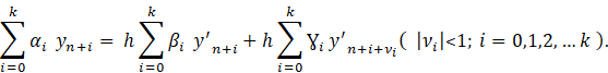
This method has investigated by many authors (see for example [15]-[20]). By this method one can be solved ODEs, Volttera integral and Volttera integro-differential equations.

In application of this method are arises some difficulties. Therefore, here also to consider the case k=1, it is easy to understand, that constructed simple methods, which have applied to solve model problem. For this let us consider to the following method: 

 

           ).              Equation 7

 

It is known that the coefficient in this formula can be chosen so that degree p=6.

Let’s  simplify this method and explore it in two versions.

First, let us consider following method:

 

Equation 8

 

By choosing the coefficients, 𝛼 and 𝛽 one can constructed method with the order of accuracy p>2 (as is known the method with the order accuracy p=2 is the trapezoidal rule, which is very popular) and can be receive from the formula Equation 7 in the case . It is known that, by choosing the coefficients, 𝛼 and 𝛽, one can be constructed by hybrid method with the order of accuracy p=4, but in this case values of constant 𝛼 and 𝛽 will be irrational and in this case arises some difficulty with the calculation of the values   and. Therefore, here decided to take the values of 𝛼 and 𝛽-as the rational number. For example, as the midpoint rule, this can be written as:

 

,                                                      Equation 9

                                                                         

But, noted that the following hybrid method

 

)/4,                                                    Equation 10

 

has the order of accuracy p=3? Noted that method Equation 9 is explicit, but the method Equation 10 is implicit. Let us the unknowns, 𝛼 and 𝛽 choose so as method Equation 8 will be having the maximal order of accuracy. For this to consider the following Taylor series:

 

=+h𝛼+++…,

 

=+hβ+++… .

 

By using these expressions in the method of Equation 8 receive, that in order to the order of the method Equation 8 has the order of accuracy p=4, the unknowns must satisfy the following system of algebraic equations:

 

                                                                        / (j+1), j=1, 2, 3.                                          Equation 11

 

By solving this nonlinear system, receive the following solution:

 

; 𝛼= (3-)/6, 𝛽= (3+)/6.

 

If use these values in the formula Equation 8, then we receive the following method:

 

 

+                                                                 Equation 12

 

which has the order of the accuracy p=4.

It is not difficult to prove, that the above received solution of the system nonlinear equations Equation 11 is unique. Therefore method Equation 12 is also unique. But method of type Equation 10 is not unique. The following method is also having type of Equation 10

 

+                                                        Equation 13

 

Methods Equation 10 and Equation 13 different from the method Equation 12 that in the methods Equation 10 and Equation 13 has used the hybrid points of the rational type, but in the method Equation 12 have used hybrid points of the irrational type. Noted that, methods Equation 10 and Equation 13 have the degree p=3.

It is easy to understand, that to calculation of the values  and  is not easy, so as 𝛼 and 𝛽 are the irrational numbers. Therefore some scientists suggested using the values with type , here m and l are the rational numbers. The methods Equation 9 and Equation 10 are of this type. And now let us show that for using values like, can be use the value , which can be calculated by fractional step size h/m. Methods Equation 9 and Equation 10 are the methods with fructional step size. Let us consider application them to solving some problem. It is obvious that for the application to solve some problem it is necessary to construct some methods for calculation of the walk . By taking into account that the transaction error for this method can be presented as O (). It follows from here, that the value  must be calculated with the local transaction error O (). In this case method Equation 9 can be using in the following form:

 

 

                                                        

 

Here has used the explicit Euler method. To obtain more accurate calculations, one could use the implicit Euler method. And now let us consider to application of using method Equation 10 one must use more accurately methods. If take into account that the order of the accurate for the method can be written as: p=3, then receive that constructed methods for calculation of value the  must had the accuracy p≥2. Hence for calculation of the value  one can be used the method Equation 9 or the trapezoidal rule. Thus, there have shown, that the methods with the fractional step-size have some advantages.

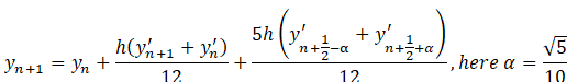
For the illustration of above mention let’s consider using the following way:

 

                                            Equation 14

 

Here we have used the values, calculated by the methods Equation 10 and Equation 13. It is clear, that by using methods Equation 14 one can be calculated the approximately values of our problems at the mesh point  . It is easy to understand, that the values of the solution of our problems calculated by the method Equation 14 will be more exact, than the values, calculated by the methods Equation 10 and Equation 13. By taking into the account the local transaction error of the methods Equation 10, Equation 13 and Equation 14 we receive, that methods Equation 10 and Equation 13 have the degree p=3, but the method Equation 14 will have the degree p=4. It is obvious, that method Equation 14 is more exact. Let us note that the methods Equation 10 and Equation 13 can be taken as the symmetric methods. Therefore, above constructed methods can be taken as the bilateral methods. It follows from here, that by using methods Equation 10 and Equation 13 one can be defining the interval in which located the exact values of the solution considering problem, which is very basic question in solving practical problems.

 

4. NUMERICAL RESULTS

For the illustration above received theoretical results, let us consider applications of the methods Equation 10, Equation 13, Equation 14 to following Volterra integral equation of the second kind:

 

 Equation 15

 

the exact solution of the equation equals

 

 

Table 1 The Errors of Methods For
	h=0.1			h=0.05
	For the Equation 10	For the Equation 13	For the Equation 14	For the Equation 10	For the Equation 13	For the Equation 14
0.1	4.39E-7	4.42E-7	1.47E-9	5.49E-8	5.52E-8	9.18E-11
0.3	1.19E-6	1.20E-6	3.99E-9	1.49E-7	1.50E-7	2.49E-10
0.5	1.82E-6	1.83E-6	6.07E-9	2.27E-7	2.28E-7	3.79E-10
0.8	2.54E-6	2.56E-6	8.50E-9	3.18E-7	3.19E-7	5.31E-10
1	2.92E-6	2.94E-6	9.75E-9	3.65E-7	3.66E-7	6.09E-10

 

By using the values  receive that, this solution of our problem will be decreasing. Therefore, in the following table located the values of our problem Equation 15, calculated by the methods Equation 10, Equation 13 and Equation 14.

Table 2 The Errors of Methods For
	h=0.1			h=0.05
	For the Equation 10	For the Equation 13	For the Equation 14	For the Equation 10	For the Equation 13	For the Equation 14
0.1	4.88E-7	4.85E-7	1.62E-09	6.09E-08	6.07E-8	1.01E-10
0.3	1.62E-6	1.63E-6	5.39E-09	2.03E-07	2.02E-7	3.37E-10
0.5	3.01E-6	2.99E-06	1.00E-08	3.76E-07	3.75E-07	6.26E-10
0.8	5.69E-06	5.65E-06	1.89E-08	7.10E-07	7.07E-07	1.18E-09
1	7.98E-6	7.93E-06	2.65E-08	9.96E-07	9.93E-07	1.66E-09

 

By the comparison results, located in the table Table 1 and Table 2 receive, that if the solution, investigated problem Equation 15 is increasing in this case the approximately value is also increase to corresponding exact values.

Table 3 The Errors of Methods For
	h=0.1			h=0.05
	For the Equation 10	For the Equation 13	For the Equation 14	For the Equation 10	For the Equation 13	For the Equation 14
0.1	0.0002	0.0003	3.77E-06	2.82E-05	2.87E-05	2.37E-07
0.3	0.0004	0.0005	7.44E-06	5.56E-05	5.66E-05	4.67E-07
0.5	0.0005	0.0006	8.79E-06	6.57E-05	6.68E-05	5.52E-07
0.8	0.0005	0.0006	9.40E-06	7.02E-05	7.14E-05	5.90E-07
1	0.0005	0.0006	9.52E-06	7.11E-05	7.23E-05	5.97E-07

 

For the receiving more exact compare the values, calculated by the methods Equation 10, Equation 13, Equation 14 for ⋋=-5 and for h=0.1 and h=0.05 in the Table 3 we have located the values, calculated by above mentioned methods.

Table 4 The Errors of Methods For
	h=0.1			h=0.05
	For the Equation 10	For the Equation 13	For the Equation 14	For the Equation 10	For the Equation 13	For the Equation 14
0.1	0.0003	0.0003	6.22E-06	4.72E-05	4.64E-05	3.90E-07
0.3	0.002	0.0019	3.33E-05	0.0002	0.0002	2.09E-06
0.5	0.0065	0.0063	0.00018	0.0008	0.0008	6.72E-06
0.8	0.0313	0.0302	0.00051	0.0039	0.0038	3.22E-05
1	0.0861	0.0833	0.00141	0.0107	0.0105	8.87E-05

 

By continioing the above described tables in table Table 4 have used values, calculated with the application above mentioned methods, receive that results located in all the tables are corresponding to the theoretical results.

 

5. CONCLUSION

One of the well-researched numerical methods is the multistep method with constant coefficients. Recent time there is some modification of this method as the multistep advanced method or multistep hybrid methods. One of the disadvantages of these methods is the calculation the values of the solution of the investigated problem at the irrational mesh points. To construct a method freed from the specified flaw, here has recommended replacing the values of   with the rational number and have shown that, in this case how one can be modified of the known for methods for the calculation of the values. In this case we receive the fractional step method. The well-known representatives of these methods are the midpoint rule. As shown in the text to construct suitable methods for calculating values of the solution our problem at the fractional steps is not difficult. Note that, the numerical methods with fractional steps have investigated by academician Yanenko. But the way, which have presented here to construct the methods with the fractional step-size differ from above mentioned methods in that this scheme is very simple. Noted, that the stable hybrid methods are more exact than the stable methods with fractional step-size. As was noted above by using the results, receiving by the symmetrical methods one can be locate the exact values of the solution of solving problem. Given the specified properties of these methods one can be increase the order of accuracy the values, calculated by the linear combination of these methods. This can be confirmed by the results of solving our example. We believe that this method will find its followers.

 

ACNOWLEDGMENTS

The author expresses thank to the academician Medieval Galina Yuryevna for her suggestion to investigate to the computational aspects of our problem.

 

REFERENCES

ButcherJ.C. (1965) A modified multistep method for the numerical integration of ordinary differential equations. J. Assoc. Comput. Math., v.12, pp. 124-135. Retrieved from https://doi.org/10.1145/321250.321261

Gear C.S., (1965) Hybrid methods for initial value problems in ordinary differential equations, Algorithm IS, J. Number. Anal. v. 2, pp. 69-86. Retrieved from https://doi.org/10.1137/0702006

Hairier E., Norsett S.P., Wanner G. (1990) Solving ordinary differential equations. (Russian) М., Mir, Retrieved from https://doi.org/10.1007/978-3-662-09947-6

Ibrahimov V.R. ; Imanova M.N. (2021) Multistep methods of the hybrid type and their application to solve the second kind Volterra integral equation, Symmetry 6 13. Retrieved from https://doi.org/10.3390/sym13061087

IbrahimovV.R. (1984) Convergence of the predictor-corrector methods, Godishnik na Vischite uchebzaved. Applied Mathematics, Sofia Boolgaria, pages 187-197

Imanova M.N. (2020) On some comparison of Computing Indefinite integrals with the solution of the initial-value problem for ODE, WSEAS Transactions on Mathematics, 19.19. Retrieved from https://doi.org/10.37394/23206.2020.19.19

Imanova M.N. (2020) On the comparison of Gauss and Hybrid methods and their application to calculation of definite integrals, MMCTSE, Journal of Physics; Conference Series, DOI 10.1088/1742-6596/1742-6596/1564/1/012019, 1564(2020)012019.  Retrieved from https://doi.org/10.1088/1742-6596/1564/1/012019

Mehdiyeva G.Yu. (n.d.) ; Ibrahimov V.R On the Computation of Double Integrals by Using Some Connection Between The Wave Equation and The System Of ODE. Retrieved from  https://www.researchgate.net/profile/Vagif-Ibrahimov/publication/350755242_On_The_Computation_Of_Double_Integrals_By_Using_Some_Connection_Between_The_Wave_Equation_And_The_System_Of_ODE/links/607019f44585150fe993e059/On-The-Computation-Of-Double-Integrals-By-Using-Some-Connection-Between-The-Wave-Equation-And-The-System-Of-ODE.pdf

Mehdiyeva G.Yu. ; Ibrahimov V.R. ; Imanova M.N. (2019) On the construction of the advanced Hybrid Methods and application to solving Volterra Integral Equation, WSEAS Weak transactions on systems and control, V.14.

Mehdiyeva G.Yu. ; Ibrahimov V.R.;X.-G.Yue, M.K.A.Kaabar, S.Noeiaghdam, D.A.Juraev, (2021)Novel symmetric mathematical problems, international journal of circuits, Systems and signal processing 15  1545-1557. Retrieved from https://doi.org/10.46300/9106.2021.15.167

Polushuk E.M. (1977), Vito Volterra, Nauka, Leningrad, ,114 p.

Verjibitskiy V.M. (2001), Numerical methods, Moscow, Visshaya Shkola, ,382

Verlan A.F., Sizikov V.S. (1986), Integral equations methods, Naukova Dumka, Kiev, 543 p.

Volterra V. (1982), Theory of functions and of integral and integro-differential equations, Moscow, fiz-mat., literature, 304 p