No work has compared performance of five GARCH type models for Nigerian stock exchange. Therefore, this current study will compare the performance of GARCH type models, ascertain the best fit model, estimate parameters and make forecast with the optimal model.

 

2. LITERATURE REVIEW

 Vitor (2015) employed GARCH family models to investigate the sensitivity of shock persistence and asymmetric effects in the international stock market during the global financial crises using daily data of twelve stock indexes over the period from October 1999 to June 2011. The results showed that the Subprime crisis period turned out to have bigger impact on stock market volatility with high shock persistence and asymmetric effects.

 Tabajara et al.   (2014) compared the stock market behaviour of Brazil, Russia, India and China (BRIC) emerging economies to those of the industrialized economy of USA, Japan, United Kingdom and Germany in the light of 2008 global financial crisis using GARCH, EGARCH and TARCH univariate models. The stock market behaviours of the BRIC’s emerging markets and the industrialized economies in terms of shock persistence effects on volatility, asymmetry and delayed reaction of volatility to stock market changes were found to be similar in both markets. However, the BRIC’s stock markets showed less persistence of shocks, less asymmetric effects and faster volatility reactions to market changes.

Ding et al.  (1993) extended the standard deviation GARCH model proposed by Taylor (1986) and Schwert (1989) named Power GARCH (PGARCH). This model multiplies the power of the conditional standard deviation d (positive exponent) with the function of the lagged conditional standard deviation and lagged absolute innovation. When the positive exponent is set to 2, this expression becomes the standard GARCH model. The provision of switching power supplies increases the flexibility of the model.

Miron   and Tudor (2010) studied several types of asymmetric GARCH models (EGARCH, PGARCH, and TGARCH) using the stock indexes of the United States and Romania from 2002 to 2010. They proved that the estimation of volatility comes from the application of the EGARCH model and is more reliable than the estimation of other models. EGARCH records the asymmetry between returns, volatility and aims to compensate for the three main shortcomings of the GARCH model. (i) Ensuring the parameter constraints of positive conditional variance; (ii) Insensitive to the asymmetric response of volatility to shocks; and (iii) It is difficult to measure persistence in highly stable series. The logarithm of the conditional variance in the EGARCH model means that the leverage is exponential rather than quadratic. Specifying the volatility in the form of logarithmic transformation means that the parameters are unrestricted to ensure the positiveness of the variance (Majose, 2010), which is the decisive advantage of the EGARCH model over the symmetric GARCH model.

Chang (2010) analyzes the effect of the economic and financial crisis on Chinese stock return volatility using daily data from 2000 to 2007 as the pre-crisis period and 2007 to 2010 as the during crisis period. The findings show that the EGARCH model fits the data better than the GARCH model in modeling the volatility of Chinese stock returns. The result also indicated that volatility is more persistent during crisis period than in pre-crisis period.

Aliyu (2011) assessed the innovations of monetary policy in Nigerian stock market during the global financial crisis period using monthly data for the period of January 2007 to August 2011. He employed EGARCH model and regressed stock market returns against money stock (M1 and M2) and monetary policy rate (MPR). The empirical findings from the study revealed that, unlike the anticipated components of the monetary innovation, the unanticipated component of the policy innovations on M2 and MPR exerted destabilizing effect on Nigerian stock returns.

Franses   and Van Dijk (1996) compared three models of the GARCH family (GARCH, QGARCH, and GJRGARCH) to predict the weekly volatility of several European stock indexes. At the end of this study, they found that the non-linear model could not beat the standard GARCH model.

Jayasuriya (2002) examined the effect of stock market liberalization on stock returns volatility in Nigeria and fourteen other emerging market data, from December 1984 to March 2000 to estimate symmetric GARCH model. The study found that positive (negative) changes in prices have been followed by negative (positive) changes in volatility. The Nigeria portion of the result indicates more of business cycle behavior of stock return rather than volatility clustering. In studying volatility behavior of stock returns for emerging markets, Ogum et al. (2005) apply the Nigerian and Kenya stock data on EGARCH model. The finding differed from that of Jayasuriya (2002). Although volatility persistence was found in both markets; volatility responds more to negative shocks in the Nigeria market and the reverse is the case for Kenya market.

 

3. MATERIAL AND METHODS

3.1. METHOD OF DATA COLLECTION

The study used secondary data and is all about UBA daily stock exchange prices in Nigeria. The dataset used for this study was collected from the official websites of www.investing.com,on the daily basis of the Nigeria stock exchange rate over a period of ten years. (06/06/2012 – 04/06/2021).

 

3.2. METHODS OF DATA ANALYSIS

3.2.1.  AUGMENTED DICKEY-FULLER TEST (ADF) 

The Augmented Dickey-Fuller (ADF) test was employed in the study. This is an augmented version of the Dickey Fuller test for data which is considered large and complicated for time series models. The testing for ADF is similar to the Dickey-Fuller and can be applied to the regression model:

 

∆𝑦_𝑡 = + + 𝜃𝑦_𝑡−1 + 

                                                                                                          

Where ∆ is difference operator, 𝛽₀ is the constant, is the coefficient on a time trend and 𝛾_𝑖 is the lag of autoregressive process, and 𝑎_𝑡 is error term.

The hypothesis formulated  

H₀: =1 (There is unit root)

H₁:< 1(There is no unit root)                             

 The ADF test statistic is given by 

 

ADF =

 

Where  denotes the least square estimate of 𝛾 is as well know Augmented Dickey fuller test.

The null hypothesis of the unit root is accepted if the p-value is greater than critical value.

 

3.3. MODEL OF SELECTION CRITERION

3.3.1.  AKAIKE INFORMATION CRITERION (AIC) 

The Akaike Information Criterion (AIC) is a measure of the relative goodness of fit of a statistical model. Akaike (1974) suggested that the goodness of fit of a given model should be measured by weighing the fitting error and the number of parameters in the model. When a specific model is used to describe reality, it provides a level of information loss. Given a data, several competing models may be ranked according to their AIC, with the one having the lowest AIC being the best model.

Mathematically, 

 

The AIC is defined as     = 2(k−In(L)                                                                       3.3

 

When k is the number of parameters in the statistical model, and L is the maximized value of likelihood function for the estimated model.

 

3.3.2.  BAYESIAN INFORMATION CRITERION

Bayesian Information criterion (BIC) or Schwarz Criterion is a criterion for model selection among parametric model classes with different parameters. Choosing a model to optimize BIC is a form of regularization. BIC assumes that the data distribution is an asymptotic result of the exponential distribution. Mathematically expression

 

Let    BIC =-2𝑙𝑜𝑔_𝑒L +K𝑙𝑜𝑔_𝑒n                                                                                       3.4

 

Where n = sample size, k = the number of free parameters to be estimated L = the maximized value of the likelihood function for the estimated model. In this study ADF will employed in this paper

 

3.4. TEST FOR NORMALITY  

The test for normality is done using the Jarque-Bera test statistic. According to Dikko et al. (2015), Jarque-Bera could be defined as points test of skewness and Kurtosis to examine whether data series exhibit normal distribution or not. The test statistics was developed by Jarque   and Bera (1980).  and this is defined as

Test statistic:

 

                      J B =                                                                                   3.5

 

Where n = sample size, S= skewness coefficient, and K =kurtosis. Under the null hypothesis of a normal distribution, the Jarque-Bera statistic is distributed as with 2 degrees of freedom. The probability that a Jarque-Bera statistic exceeds (in absolute value) the observed value under the null hypothesis—a small probability value leads to the rejection of the null hypothesis of a normal distribution. 

 

3.5. TEST FOR RANDOMNESS

The adequacy of the GARCH model implies that any of a group of autocorrelations of a time series is different from zero. The test investigates the overall randomness based on a number of lags. Ljung–Box (Ljung and Box 1978) test is employed in this research to test for the adequacy of the optimal GARCH family model. The Ljung–Box statistic is defined as  

 

           Q

 

Where n is sample size, is the sample autocorrelation at lag k and h is the number of the lags being tested. 

         

3.6. TEST HETEROSCEDASTICITY (ARCH)

In this study, we employ the use of ARCH effect test. ARCH LM was proposed by Engle (1982). ARCH LM test is a langrage multiplier test to assess the significance of ARCH effect. Hence, the conditional heteroscedasticity in a variance is equal to the autocorrelation in the squared innovation process, is given by the regression equation

 

                                                3.7

 

Where  is a white noise error process and lag 𝑚 is a pre-specified positive integer? The null hypothesis is

 

𝐻₀: ∝₀=∝₁=, ⋯, ∝_𝑚= 0

 

The null hypothesis state that there is no ARCH effect (since the p-value is greater than the chosen significance level at 5%) Do not rejected the null hypothesis, there we conclude that there is no ARCH effect in time series.

 

3.7. ESTIMATION OF GARCH MODEL WITH DISTRIBUTION ERROR

 Several methods of error distributions we be comparing in the estimate of GARCH family model (symmetric and Asymmetric). We introduced normal, student t- distribution (std), generalized error distribution to analyze the GARCH family models using the daily UBA log return stock exchange in Nigeria. In this paperwork, we employed student t- distribution.

 

3.7.1.  NORMAL DISTRIBUTION

Standard normal error distribution the random variable (Z) following log-likelihood function needs to be maximized

 

 

 

3.7.2.  STUDENT T DISTRIBUTION ERROR

According (Shamiri and Isa, 2009), the probability density function of   is given asstandardized Student t- distribution (std)

 

 f                  -                                             3.9

 

Where ν is the number of degrees of freedom and Г denotes the Gamma function.

 

3.7.3.  GENERALIZED ERROR DISTRIBUTION

Generalized Error Distributionas proposed by Nelson (1991) is more interesting in terms of satisfying stationarity compared to the student-t distribution. Just like in the case of the student’s-t error distribution the unconditional means and variances may not be finite in the EGARCH. The log-likelihood function for the standard generalized error distribution is defined as

 

)           3.10

 

                                                                                                                 3.11

 

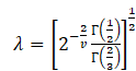
The generalized error distribution (GED) incorporates both normal error distribution when (V = 2), Laplace distribution when (v = 1), and the unique distribution for v = .

 

GARCH models

In the study, we used the univariate GARCH family model approach and also compared the different GARCH family models in analyzing the daily UBA stock exchange in Nigeria, which are indicated as follows; EGARCH, SGARCH, TGARCH or GJRGARCH, APARCH and IGARCH models

 

3.8. ARCH/GARCH FAMILY MODELS

The autoregressive conditional heteroscedastic (ARCH) model of Engle (1982), the generalized ARCH (GARCH) model of Bollerslev (1986). ARCH models which report the conditional variance, which depend on past return is that the shock at of an asset return is serially uncorrelated, but dependent,

The ARCH(q) model can be expressed as

 

                                             =

 

 

  

 

Where ~N (0,1) is a white noise process; 𝜇 is the constant mean of the returns. The conditional variance,  is a function of past squared residuals of returns, which scales the process .

In the ARCH (q) process proposed by Engle (1982),

 

3.12

 

Where  and  implied that  is strictly positive;   is the error of return estimation at time t. With these non-negative restrictions (particularly 𝜔> 0), if a major shock happened one-lagged period, two-lagged period or up to j periods ago, the impact would increase recent conditional variance. However, no matter the market movement is positive or negative, due to the squared return shock on the right-hand side

 

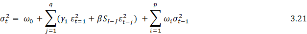
3.8.1.  GENERALIZED AUTOREGRESSIVE CONDITIONAL HETEROSKEDASTICITY (GARCH) MODEL

The standard GARCH model is proposed by Boleslaw (1986) to solve the problematic caused by the long lag structure in the ARCH process. Now GARCH (p, q) process, the conditional variance depends not only on q lagged error square, but also on p lagged historical conditional variances. The GARCH Model can be defined as the follows

 

 

is a discrete – time stochastic defined to be =𝑍_𝑡𝜎_𝑡    give   𝑍_𝑡 ~ iid. N (0,1) and 𝜎_𝑡 is the conditional standard deviation of return at time t. All parameters 𝜔, 𝛼_{1, 𝛽1} are non-negative. The stationary condition of 𝛼 + 𝛽 < 1 should hold to ensure weakly stationarity of GARCH process.

𝛼₁ indicate the short-run persistency of shock while   𝛽 implies the long run persistency

 

3.8.2.  INTEGRATED GENERALIZED AUTOREGRESSIVE CONDITIONAL HETEOSKEDASTICITY (IGARCH) MODEL

Integrated generalized autoregressive conditional heteroscedasticity (IGARCH) model. IGARCH model are unit root GARCH model. Similar to ARIMA models, a key feature of IGARCH model is that the impact of past squared shocks.for is persistent. The volatility processes in these markets are purely random walk. Therefore, IGARCH is introduced to use for such kind of non-stationary volatility process. The IGARCH (1, 1) model is specified in Tsay (2005) and Grek (2014) as

 

                                                            3.14

 

Where, Ali (2013) used  to denote. The model is also exponential smoothing for the  series. To rewrite this model as

 

 

 

 

By substitution,

 

 

Which is the well-known exponential smoothing formulation with  being the discounting factor (tsay,2005)

 

3.8.3.  THRESHOLD GENERALIZED AUTOREGRESSIVE CONDITIONAL HETEROSKEDASTICITY (TGARCH) MODEL

Threshold GARCH has been developed by Zakoian (1990) and Glosten et al.   (1993) it is also known as GJR GARCH. This model defines the conditional variance as a piecewise function and captures the asymmetric effect Zhang (2016). 

TGARCH (p, q) model specification for conditional variance is given by

 

 

where_𝑡−1 if _𝑡²< 0 and 0 otherwise

In TGARCH model, good news implied that and bad news implies that and these two shocks of equal size have differential effect on the conditional variance. Good news has an impact of 𝛼_𝑖, and bad news has an impact of 𝛼_𝑖 + 𝛾_𝑖. Bad news increase volatility when 𝛾_𝑖 > 0, which implied the existence of leverage effect in the i-th other and when 𝛾_𝑖 ≠ 0 the news impact is asymmetric. However, the first order representation is of TGARCH (p, q) is 

 

 

3.8.4.  GLOSTEN-JAGANATHAN AND RUNKLE GENERALIZED AUTOREGRESSIVE CONDITIONAL HETEROSKEDASTICITY (GJR GARCH) MODEL

The GJR GARCH model is another non-linear extension of the standard GARCH model and was first proposed by Glosten et al.   (1993) and have developed the GJR –GARCH model which estimates effect of good news and bad news in financial stock markets. Therefore, to take into account this kind of effect, a dummy variable is introduced into the symmetric GARCH model. This model covers asymmetric or leverage effect confidently a with long memory.

 

GJR-GARCH model can be expressed as

 

 

where S, is a dummy variable that takes the value "1" when the error term and 1 is negative and

"O" and when the error term is positive Raza et al.   (2015).

 

3.8.5.  Exponential Generalized Autoregressive Conditional Heteroskedasticity (EGARCH)Model 

Exponential GARCH (EGARCH) model of was proposed by Nelson (1991) There are various ways to express the EGARCH model. However, it allows for asymmetric effects between positive and negative asset returns, he considered the weighted innovation.

The EGARCH specification as specifies log volatility as

 

 

Where is iid with a generalized error distribution (GED) which nest the Gaussian and allow for slightly fatter tail. Due the specification of log volatility, no parameter restriction is necessary to keep volatility positive. However, the condition for weak and strong stationarity coincides. Here, that if 𝜃 = 0, then Cov (𝑦_𝑖², 𝑦𝑡_−𝑗) ≠ 0 such that a leverage effect can be captured

 

3.8.6.  ASYMMETRY POWER AUTOREGRESSIVE CONDITIONAL HETEROSKEDASTICITY (APARCH) MODEL

Asymmetry power ARCH(APARCH) model was developed byDing et al.   (1993).

 PGARCH (p, q) it can mathematical written as  

 

                                          3.23

 

Note, 𝛿> 0 𝑎𝑛𝑑ℝ⁺, < 1 establish the existence of leverage effect. If 𝛿 = 2, the PGARCH (p,q) replicate  a GARCH(p,q) with a leverage effect. If 𝛿 = 1, standard deviate is modeled.

The first order PGARCH can be mathematical equation

 

 

The failure to accept the null hypothesis that 𝛾_𝑖 ≠ 0, shows the presence of leverage effect. The impact of news on volatility in PGARCH is similar to that of TGARCH when 𝛿 𝑖𝑠 1

 

4. DATA ANALYSIS AND RESULTS

 The plot time showed the direction of movement of the daily stock exchange prices in Nigeria over the period of ten years

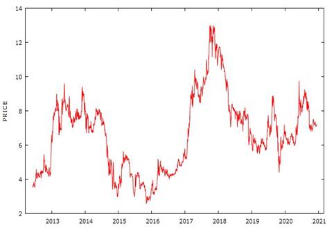
Figure 1

 

Figure 1 present the original time plot of daily stock price in Nigeria (UBA). The plot shows the movement of daily stock prices over period of time between 2012-2021.The data exhibits the presence of persistence, trend and non-stationary in the observed data. The stock price rose steadily to peak level in the middle of 2013, maintaining its fluctuation till the middle of 2013 and 2014, it finally dropped at 2015/2016. Later, between 2017 there is fluctuation in stock price. It also maintained a peak level between 2017/2018, at beginning 2018 the stock price starting decline.

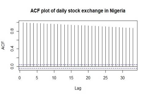
Figure 2

 

 

 Figure 2 Present the ACF plot of Daily Stock Exchange Price in Nigeria (UBA), it can be observed from the autocorrelation function plot, the data decaying slowly and non-stationary.

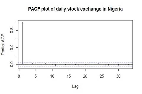
Figure 3

 

Figure 3 present PACF plot of Daily Stock Exchange Price in Nigeria (UBA), it can be observed from the partial autocorrelation function plot, that the data is sinuous in nature and non-stationary.

 

4.1. RESULT OF ROOT TEST

 The ADF test is (-2.1001), at the chosen level of significance (0.05), the p-value of the test (0.5359) is greater than 0.05. The null hypothesis is not rejected. This implies that, Nigeria’s daily stock exchange price is non-stationary.

 

Table 1 Descriptive statistics of daily price and log return in Nigeria 2012-2021
Statistics	DSE prices	DSE log return prices
Number of observations	2225	2224
Minimum	2.59	-0.042324
Maximum	13	0.088493
Mean	6.638908	-0.000138
Median	6.75	0
Sum	14771.57	-306531
Standard deviation	2.202832	0.012671
Skewness	0.414509	0.012671
Kurtosis	-0.2299624	4.267005

 

Show the summary descriptive statistics for the daily stock exchange price and log return series. The skewness is 0.285355 for the return series and 0.414509 for the daily stock price. And this is an indication of a positive skewness. This implies that most of the values of the series are concentrated on the right side of the mean. Furthermore, kurtosis value (4.267005) is greater than that of normal distribution which is 3. It shows that the distribution has a fat tail and also indicates the distribution has a small outlier. On the contrary, the kurtosis value (-0.229624) is less than that of normal distribution. It shows that the distribution has a flat tail which is one of the (features) of stock returns.

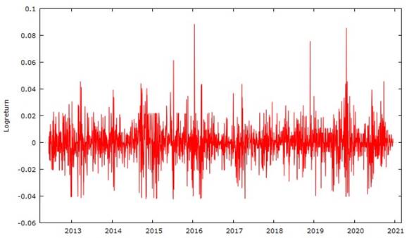
Figure 4

 

Figure 4 present the plot of the stationary of DSE log return. The variance and mean of this series are now fluctuating around a common location with no indication of structural breaks. The time plot we observe that the returns vary along the zero line with the largest log return of stock prices observed around 2013,2015, 2016 and 2019 having a value of -0.04, while 2017 having value -0.05. During the years 2016, 2019-2020, there is spike in volatility indicating non-constant conditional volatility

 

4.2. RESULT OF TEST OF RANDOMNESS (LJUNG-BOX TEST)

statistic (Chi-squared) = 19.301, df = 1, p-value =1.116e-05

Conclusion: The daily log return price auto correlated at 5% level of significance.

 

4.3. Test for Heteroskedasticity (ARCH LM) test

Test statistic (Chi-squared) =247.26, Degree freedom=100, p-value=1.792e-14

Conclusion: Since the p-value (p-value=2.2e-16) is less than 0.05, Therefore we reject the null hypothesis and conclude that is there is an ARCH effect presence

 

4.4. Fitting of the GARCH series (symmetric and asymmetric) family models

 

Table 2 Present ARMA (0,0)- SGARCH (1,1,) with different Distribution error
Normal
Model	Parameter	Estimate	Pr(>|t|)	AIC	BIG	MLE
SGARCH (1,1)		-0.000033	0.8854	-6.0688	-6.0577	6148.632
		0.000024	0
		0.269099	0
		0.597631	0
Student’s t distribution
Mode	Parameter	Estimate	Pr(>|t|)	AIC	BIC	MLE
SGARCH (1,1)		0.000098	0.602714	-6.1784	-6.1645	6260.621
		0.000019	0.000046
		0.370307	0
		0.611955	0
Generalize error distribution
Model	Parameter	Estimate	Pr(>|t|)	AIC	BIC	MLE
SGARCH (1,1)		0	0.999959	-6.2178	-6.2039	6300.524
		0.000019	0.000239
		0.364403	0
		0.617922	0

 

Table 3 Present ARMA (0,0)- APARCH (1,1,) with different Distribution error
Normal Distribution
Model	Parameter	Estimate	Pr(>|t|)	AIC	BIC	MLE
APARCH (1,1)		-0.000131	0.579306	-6.0631	-6.0465	6144.909
		0	0.437921
		0.210776	0
		0.553791	0
		0.06902	0.049151
		3.185452	0
Student’s t distribution
Model	Parameter	Estimate	Pr(>|t|)	AIC	BIC	MLE
APARCH (1,1)		0.000056	0.77202	-6.1769	-6.1575	6261.122
		0.000042	0.5035
		0.361589	0
		0.622841	0
		0.038706	0.43348
		1.830679	0
Generalize error Distribution
Model	Parameter	Estimate	Pr(>|t|)	AIC	BIC	MLE
APARCH		0	1	-6.1871	-6.1677	6271.466
		0	0.80291
		0.056049	0
		0.892102	0
		0.064414	0.301
		2.765914	0

 

Table 4 Present ARMA (0,0)- Gjr-GARCH (1,1,) with different Distribution error
Normal
Model	Parameter	Estimate	Pr(>|t|)	AIC	BIC	MLE
GjrGARCH (1,1)		-0.000131	0.58348	-6.0688	-6.0549	6149.665
		0.000025	0
		0.23531	0
		0.597383	0
		0.061727	0.15275
Student’s t Distribution
Model	Parameter	Estimate	Pr(>|t|)	AIC	BIC	MLE
GjrGARCH (1,1)		0.00006	0.758414	-6.1778	-6.1611	6260.998
		0.00002	0.000039
		0.338261	0.000001
		0.611086	0
		0.060385	0.389174
Generalize Error Distribution
Model	Parameter	Estimate	Pr(>|t|)	AIC	BIC	MLE
GjrGARCH (1,1)		0	1	-6.1705	-6.1705	6253.601
		0	0.8053
		0.08859	0
		0.915618	0
		-0.023208	0.11747

 

Table 5 Present ARMA (0,0)- IGARCH (1,1,) with different Distribution error
Normal
Model	Parameter	Estimate	Pr(>|t|)	AIC	BIC	MLE
IGARCH (1,1)		-0.000102	0.64349	-6.0554	-6.0471	6134.062
		0.000018	0
		0.393722	0
		0.606278	Na
Student’s t distribution
Model	Parameter	Estimate	Pr(>|t|)	AIC	BIC	MLE
IGARCH (1,1)		0.000098	0.599815	-6.1793	-6.1682	6260.551
		0.000019	0.000064
		0.386911	0
		0.613089	Na
Generalize Error Distribution
Model	Parameter	Estimate	Pr(>|t|)	AIC	BIC	MLE
IGARCH (1,1)		0	0.999721	-6.2187	-6.2076	6300.449
		0.000019	0.000142
		0.384428	0
		0.615571	Na

 

Table 6 Present ARMA (0,0)- EGARCH (1,1,) with different Distribution error
Normal
Model	Parameter	Estimate	Pr(>|t|)	AIC	BIC	MLE
EGARCH (1,1)		-0.000284	0.23213	-6.0564	-6.0425	6137.059
		-1.631956	0
		-0.02403	0.25277
		0.81224	0
		0.433991	0
Student’s   t Distribution
Model	Parameter	Estimate	Pr(>|t|)	AIC	BIC	MLE
EGARCH (1,1)		0.000074	0.697497	-6.1714	-6.1548	6254.573
		-1.188998	0.000017
		-0.020313	0.48702
		0.863507	0
		0.521023	0
Generalize Error Distribution
Model	Parameter	Estimate	Pr(>|t|)	AIC	BIC	MLE
EGARCH (1,1)		0	0.999997	-6.2129	-6.1963	6296.562
		-1.186107	0.000115
		-0.022655	0.485002
		0.864843	0
		0.512627	0

 

Table 2, 3, 4 , 5, 6 show the results obtained from the estimation of GARCH family model with their corresponding error distribution

 

 

 

 

4.5. MODEL SELECTION 

 

Table 7 shows the information criterion (AIC and BIC) of different GARCH models with three different distribution error for the models
Information criterion
Model	AIC	BIC
SGARCH (1,1) Norm	-6.0658	-6.0577
SGARCH (1,1) Std	-6.1784	-6.1645
SGARCH (1,1) Ged	-6.2178	-6.2039
APARCH (1,1) Norm	-6.6031	-6.0465
APARCH (1,1) Std	-6.1769	-6.1575
APARCH (1,1) Ged	-6.1871	-6.1677
GjrGARCH (1,1) Norm	-6.0688	-6.0549
GjrGARCH (1,1) Std	-6.1778	-6.1611
GjrGARCH (1,1) Ged	-6.1705	-6.1538
IGARCH (1,1) Norm	-6.059	-6.0451
IGARCH (1,1) Std	-6.1793	-6.1682
IGARCH (1,1) Ged	-6.2187	-6.2076
EGARCH (1,1) Norm	-6.0564	-6.0425
EGARCH (1,1) Std	-6.1714	-6.1548
EGARCH (1,1) Ged	-6.2129	-6.1963

 

Akaike information criteria (AIC) and Bayes information criteria (BIC) for GARCH family models for some values of orders p and q. The table shows that the optimal model is obtained by using the principle of parsimony.  The principle of parsimony considers GARCH family models with the least optimal AIC. Now using akaike information criterion (AIC), we make a comparison among the different GARCH family models with the three different distribution error. In this case ARMA (0,0) - EGARCH (1,1) model with Student’s t Distribution has least optimal for daily log return UBA stock exchange rate.

 

Table 8 Estimate of parameter of ARMA (0,0)- EGARCH (1,1) model with the student’s t Distribution
Parameter	Estimate	Std Error	t-value	Pr(>|t|)
	0.000074	0.000189	0.3887	0.697497
	-1.188998	0.276515	-4.29994	0.000017
	-0.020313	0.029225	-0.69506	0.48702
	0.863507	0.031497	27.41556	0
	0.521023	0.065793	7.91908	0

 

show that all the parameters ( of this model are all significant different from zero at 5% level, except. The parameter of the shape is significant. The parameters estimate () of ARMA (0,0)-EGARCH (1,1) model are 0.000074, -1.188998, -0.020313,0.863507, and 0.51023).

The results indicate for ARMA (0,0)-EGARCH (1, 1) model the leverage effect term   is negative which shows that there is an existence of the leverage effect in future returns. When,, indicates the news impact is asymmetric, supporting the use of skewed Student-t distribution for return. Since (persistence in conditional volatility) is 0.8635072 which is close to 1, implies that volatility will take long to die in the UBA.

 

4.6. Model Adequacy (Diagnostic) checking of the estimate model

 

Table 9  Show Lung-Box test on standardized residuals of EGARCH (1,1) model with std
Number of lags	Lag1	Lag2	Lag4
Statistic	18.04	18.23	19.03
p-value	2.167× 10−05	1.294× 10−05	3.578× 10−05

 

The standardized residual test of ARMA (0,0)-EGARCH (1,1) with Student t distribution. By looking at Ljung Box test on residual, if the p-value is less than the chosen level of significance. Table 9 presents the results of Ljung-Box test. The test fails to reject the null hypothesis and conclude that there is evidence of serial autocorrelation in the standardized s residuals 

 

4.7. Test for heteroscedasticity for fitted model

 

Table 10 Show Test for ARCH effect of fitted estimate model
Number of lags	ARCH lag3	ARCH lag 5	ARCH lag 7
Statistic	2.881	3.103	3.783
p-value	0.08965	0.27514	0.37887

 

Table 10: present the ARCH LM Tests. Test for null hypothesis, since the p-values>0.05 and it has been failed to reject the null hypothesis and therefore, we conclude that there is no ARCH effect in ARMA (0,0)-EGARCH (1,1) model with Student-t distribution. This confirms that the residuals behave as a white noise process.

 

4.8. Forecasting

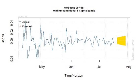
Daily UBA stock exchange price in Nigeria it has been chosen optimal model EGARCH (1,1) model with the std. The Daily UBA log return prices, which include 2225 observations for ten years, out sample data is 200. By rolling forecast method, it has been fixed length of the in-sample   period 2025 observations.

Table 11 Show the out sample of EGARCH (1,1)
Period	Series	Sigma
T+1	7.36E-05	0.006802
T+2	7.36E-05	0.007418
T+3	7.36E-05	0.007995
T+4	7.36E-05	0.008528
T+5	7.36E-05	0.009018
T+6	7.36E-05	0.009463
T+7	7.36E-05	0.009865
T+8	7.36E-05	0.010226
T+9	7.36E-05	0.010548
T+10	7.36E-05	0.010835

 

Figure 5

 

Figure 5 present the forecast plot of the ARMA (0,0)-EGARCH (1,1) model. From the forecast shows that there is no sign of fluctuation in forecast plot (ie since all the forecast plots along with the origin). There is no of volatility and clustering

 

5. CONCLUSION

This study examined the behavior of the UBA daily stock exchange prices in Nigeria for period of 2012-2021 The data was found to be with fat tail, but not stationary. Non stationarity of the data was detected using the ADF test. The data was transformed to become stationary, after the log data and also the ARCH effect test was carried out using langrage multiplier, there was heteroscedasticity. The GARCH family models were fitted to the daily log return with student -t-distribution. The ARMA (0,0)-EGARCH (1,1) model showed the best optimal model because it achieves the least AIC. It further indicated volatility clustering and leverage effect in United Bank of African (UBA) stock exchange return in Nigeria for period time. Based on the finding of this study, other time series packages should be compared with GARCH models, data should be making available for easy access and investors should be encouraged to invest in United Bank for Africa (UBA, Nigeria).

 

REFERENCES

Abdalla, S and Winker, P (2012) modeled and estimated Stock market volatility in Khartoum Stock Exchange KSE and Cairo, Alexandria Stock Exchange, CASE from Egypt.

Akaike, H. (1974). A newlook at statistical model identification. IEEE Transactions on Automatic Control, AC-19, 716-723 Retrieved from https://doi.org/10.1109/TAC.1974.1100705

Aliyu, S. U. R. (2011). Reactions of stock market to monetary policy shocks during the global financial crisis. The Nigerian Case Munich personal Repec Archive. MPRA paper No. 35581. Available online at. Retrieved from http://mpra.ub.uni.muenchen.de/35581

Bollerslev, T. (1986). Generalised Autoregressive Conditional Heteroskedasticity. Journal of Econometrics, 31 :307-327 Retrieved from https://doi.org/10.1016/0304-4076(86)90063-1

Chang, S. (2010). Application of EGARCH Model to Estmate Financial Volatility of Daily Returns : The Empirical Case of China. School of Business, Economics and Law, University of Gothenburg Retrieved from https://gupea.ub.gu.se/handle/2077/22593

Dikko, H.G., Isah. A and Chinyere S. E (2015). Modeling the Impact of Crude Oil Price Shocks on Some macro-economic Variables in Nigeria Using Generalized Autoregressive Conditional Heteroskedastic and Vector Autoregressive. American Journal of Theoretical and Applied Statistics., 6(4),12-23 Retrieved from https://doi.org/10.11648/j.ajtas.20150405.16

Ding, Z., Granger, C.W.and Engle, R.F. (1993). A long memory property of stock market returns and a new model. Journal of empirical finance, 1(1), p.83-106. Retrieved from https://doi.org/10.1016/0927-5398(93)90006-D

Engle R.F (1982). "Autoregressive Conditional Heteroskidaticity with Estimates of the Various of UK Inflation" Economical Vol. 50 No. 4 PP. 987 1008. Retrieved from https://doi.org/10.2307/1912773

Foley, S.D., (2014). The impact of regulation on market quality.

Franses, P.H. and Van Dijk, D. (1996). Forecasting Stock Market Volatility Using (Non- Linear) GARCH Models. Journal of Forecasting, 15(3), 229-235. Retrieved from https://doi.org/10.1002/(SICI)1099-131X(199604)15:3<229::AID-FOR620>3.0.CO;2-3

Glosten, L.R., Jagannathan, R. and Runkle, D.E. (1993). On the relation between the expected value and the volatility of the nominal excess return on stocks. The Journal of Finance, 48(5) : 1779-1801.  Retrieved from https://doi.org/10.1111/j.1540-6261.1993.tb05128.x

Jarque, C. M., and Bera, A. K. (1980). Efficient test for normality, heteroskedasticity and serial independence of regression residuals. Econometric Letters, 6, 255-259. Retrieved from https://doi.org/10.1016/0165-1765(80)90024-5

Jayasuriya, S. (2002). Does Stock Market Libralisation Affect the Volatility of Stock Returns ? Evidence from Emerging Market Economies. Georgetown University Discussion Series.

Kearns and A.R. Pagan (1991). Journal of Financial and Quantitative Analysis, 25 (1990), pp. 203-214. Australian stock market volatility Retrieved from https://doi.org/10.2307/2330824

Kwiatkowski, D., Phillips, P.C., Schmidt, P. and Shin, Y., (1992). Testing the null hypothesis of stationarity against the alternative of a Limit root : How sure are we that economic time series have à unit root ? Journal of econometrics, 54(1-3), pp.159-178. Retrieved from https://doi.org/10.1016/0304-4076(92)90104-Y

Miron, D. and Tudor, C. (2010). Asymmetric Conditional Volatility Models: Empirical Estimation and Comparison of Forecasting Accuracy. Romanian Journal of Economic Forecasting, 13(3), 74-92 Retrieved from https://d1wqtxts1xzle7.cloudfront.net/5236676/rjef3_10_4-with-cover-page-v2.pdf?Expires=1641618253&Signature=Kq97KDAkUFeQf5-O6jDs~PEqFvIS7gAJh7Msq66g~auWBztyBGM4wxnOAnufiJqvgb1DXVU7PN9akdcSfs8wfpHivBN2y8xMiL6o39eC1CgLaPngaM8llLn5LLOOUgu2Et57sGBHORciEaMWyQmZeIcJglX1Q-4OVsrcwB6HistTP4S0jEGftVQOkR1A2c3W~-E2Jh~5Y3TFcTnb0CtGQ3LZuMT7Ug9zLi2lAtcWoY7Q0jn9SCbmxQ29XkHwMSjQap7etpoLHFATexcvT4OYO7GafzTB~MOm5~Km4bw5dBkOm-iQqpUHaufIbVrtaNR2NddUIQ72YpQOLIbxdHEWZQ__&Key-Pair-Id=APKAJLOHF5GGSLRBV4ZA

Nelson, D. (1991). "Conditional Heteroskedasticity in Asset Returns: A New Approach", Econometrica, 59(2):347-370. Retrieved from https://doi.org/10.2307/2938260

Ogum, G. Beer, F and Nouyrigat, G. (2005). Emerging Equity Market Volatility: An Empirical Investigation of Markets in Kenya and Nigeria. Journal of African Business 6 (1/2) :139- 154. Retrieved from https://doi.org/10.1300/J156v06n01_08

Raza, M.A., Arshad, I.A., Ali, N. and Muna War, S. (2015). Empirical analysis of stock returns using symmetric and asymmetric GARH models : evidence from Karachi stock exchange. Science International, 27(1), p.795-801.

Schwert, G. W. (1989). Why does market volatility change over time ? Journal of Finance, 44 :1115-1153. Retrieved from  https://doi.org/10.1111/j.1540-6261.1989.tb02647.x

Sharmiri, A. and Isa Z. (2009). Modeling and forecasting volatility of the Malaysian Stock Markets, 2(3), 234-240 Retrieved from https://doi.org/10.3844/jmssp.2009.234.240

Spiro, P. S. (1990). Stock market overreaction to bad news in good times : A rational expectation equilibrium model. Review of Financial Studies 12 :975-1007. Retrieved from https://doi.org/10.1093/rfs/12.5.975

Tabajara, P. J., Faliano, G. L. and Luiz, E. G. (2014). Volatility behavior of BRIC capital markets in the 2008 international financial crisis. African Journal of Business management, 8(11), 373-381 Retrieved from https://doi.org/10.5897/AJBM2013.7162

Vitor, G. (2015). Sensitivity, persistence and asymmetric effects in international stock market volatility during the global financial crisis. Revista de Metodos Cuantitativos Para la Economiayla Empresa,19, 42-65. Retrieved from https://www.econstor.eu/handle/10419/113885

Zakoian, J.-M. (1994). Threshold heteroskedastic models. Journal of Economic Dynamics and control, 18(5) :93 1-955. Retrieved from https://doi.org/10.1016/0165-1889(94)90039-6

Zhang, H.K. (2016). Value-at-Risk estimation of metal market : A GED based TGARCH- EVT Approach