Doyle et al. (2004), epilepsy Khoa and Toi (2012), disorders Wajnsztejn et al. (2016), Kawe et al. (2019), magnetoencephalograms Gómez et al. (2009), Khoa and Toi (2012), neuro-physiology Kesić and Spasić (2016), electroencephalograms Paramanathan and Uthayakumar (2008), Kawe et al. (2019), Zappasodi et al. (2014), and brain entrainment Shamsi et al. (2021). The Higuchi method generally exceeds the efficiency of well-known linear methods such as the fast Fourier and wavelet transforms. Those methods work well when signals are stationary, but the increasing richness of data that are not only nonstationary but generated by non-equilibrium and noisy processes eliminates their advantages.

The Higuchi algorithm exhibits sensitive dependence on a tuning parameter k_max, defined in the following section. In the original paper Higuchi did not elaborate on the selection of the tuning parameter and for illustration used k_max=2¹¹ for time series of length N=2¹⁷. Subsequent authors used similar values for the tuning parameter but it has been discovered that the tuning parameter plays a crucial role in estimation the HFD. Several studies have addressed the issue of proper selection of tuning parameter k_max. An early paper Affinito et al. (1997) calculated HFD values for k_max=3-10 for time series ranging in length from N=50-1000, settling on k_max=6 as the optimum. The goal was to determine, in their study of electroencephalograms, the most suitable pair of (k_max, N).

Table 1 Use of Higuchi algorithm and parameters
Reference	Topic	N	kmax	N/ kmax
Higuchi (1988)	Space plasmas	217	211	64
Wajnsztejn et al. (2016)	Psychological disorder	1000	10	100
Gomolka et al. (2018)	Heart rate variability	100	5	20
Accardo et al. (1997)	EEG	50-1000	6 (3-10)	8.3-166.7
Doyle et al. (2004)	A/P gait	2400	60	40
Virkkala et al. (2002)	EEG	200	8	25
Klonowski et al. (2004)	Economics	216	15	14.4
Mujiono et al. (2013)	DNA	222	5-100	104-106
Zappasodi et al. (2014)	EEG	2560	16	160
Gómez et al. (2009)	MEG	848	48	17.7
Polychronaki et al. (2010)	Epilepsy	800	2-80	10-400

 

Decades later the literature is unclear on the method of determining the appropriate value of the tuning parameter, usually suggesting that k_max must be deter-mined on a case-by-case basis. Several papers recommend plotting the calculated HFD against a range of k_max, and selecting the appropriate k_max at the location where the calculated HFD approaches a local maximum or asymptote, considered to be a saturation point Doyle et al. (2004), Wajnsztejn et al. (2016). Gomolka et al. (2018) select k_max on the basis of statistical tests that allow discrimination between known healthy and diabetic subjects. Paramanathan and Uthayakumar (2008) proposed to determine k_max based on a size-measure relationship, that employs a recursive length of the signal from different measuring scales. In most cases researchers found that the calculated HFD is not much affected by length of the time-series but depends more strongly on k_max. Therefore, a poorly chosen tuning parameter can severely prejudice results.

Table 1 shows a sample of pairs of (k_max, N) from the literature. There is clearly no established procedure widely accepted for determining the tuning parameter. The plethora of values selected for the tuning parameter makes it clear that the community would benefit from a careful consideration of selection criteria for the tuning parameter, especially with long time-series and big data where it is impractical to examine an almost infinite number of curves of HFD against k_max.

In summary, one of main the difficulties in performing the Higuchi algorithm are that it relies on a tuning parameter, k_max, that in most cases must be selected before the fractal dimension is computed. Our goal in this paper is to explore the optimum sample pairs between the tuning parameter and length of the time series for the most general types of data.

 

2. MATERIALS AND METHODS

The Higuchi algorithm takes a signal and discretizes it into the form of a time series,  From this series we derive a new time series, , defined as follows:

 

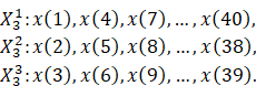
where [] represents the integer part of the enclosed value. The integer is the start time;  is the time interval, with  is a free tuning parameter. This means that a given time interval equal to , spawns -sets of new time series. For instance, if  and the time series has length , the following three time series are derived from the original data:

 

 

The length of any one of these curves is given by:

 

 

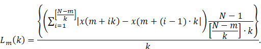
The length of the curve for the time interval  is then defined as the average over the  sets of

 

 

If this equation scales according to the rule  then the time series behaves as a fractal with dimension D. Thus, the HFD is defined as the slope of the straight line that fits the curve of ln(L(k)) versus ln(1/k).

 

 

 

 

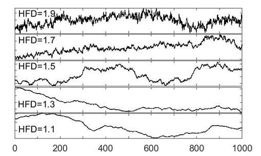
Figure 1 Sample fBm for HFD between 1.1 and 1.9.

 

The data we experiment on are theoretically derived fractional Brownian motions (fBm). fBm is a continuous-time random process proposed by Mandelbrot and John (1968). A signal that displays fBm is expressed in terms of stochastic integrals of time integrations of fractional Gaussian noise:

 

 

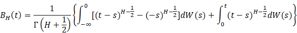
Here W is a white noise process defined on (-∞, ∞), and  is known as the Hurst parameter. The Hurst exponent for the signal is its roughness averaged over many length scales. The covariance function is given by

 

 

so that  and . This means that for the special case H=1/2, fBm reduces to the well-known random walk. The relationship between H and HFD is HFD , with values between 1 and 2. Thus, we are able to use the fBm process as our data source with a well-defined HFD in order to determine how well the Higuchi algorithm is able to accurately recover the theoretical value.

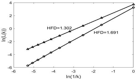
Figure 1 shows sample data of fBm signals for different values of the HFD. We create these data using a wavelet-based synthesis of fBm generation based on a biorthogonal wavelet method proposed by Meyer and Sellan Abry and Sellan (1996), Bardet et al. (2003) implemented in Matlab software. Figure 2 shows examples of how, in the Higuchi algorithm, the slope is calculated from the slope of linear fits for the curve of ln(L(k)) versus ln(1/k) for theoretical values of HFD of 1.3 and 1.7.

 

 

 

 

Figure 2 HFD is defined as the slope of the straight line that fits the curve of ln(L(k)) versus ln(1/k).

 

3. RESULTS AND DISCUSSIONS

One way that is suggested to find the optimal k_max is by plotting the calculated HFD against the k_max, and by selecting the value in the range for which HFD(k) achieves a plateau. This assumes that a plateau is achieved in every case for different classes of HFD. It is not a priori evident that this will be the case since, as is demonstrated in Figure 1, different values for the fractal dimension create time series with different roughness, which will influence the accuracy of the Higuchi algorithm. Those with HFD below 1.5 are smoother curves having clear long-range dependence while curves with higher values are rougher.

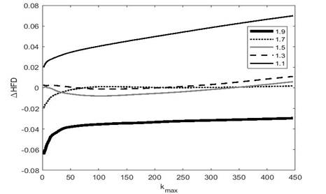
Figure 3 shows the error between the theoretical HFD and the value calculated via the Higuchi algorithm, for time series of length N=1,000, and varying values of k_max. In general, for the smallest k_max=2 the persistent time series, with HFD<1.5 produces an underestimate the theoretical fractal dimension, and antipersistent time series an overestimate. What we note here is that not every case shows the HFD estimate reaches a plateau, thus demonstrating that seeking to find the optimum tuning parameter by a plateau is not in general a valid procedure in the Higuchi algorithm. Indeed, for the persistent time series there is no plateau that is achieved. The antipersistent curves do show a clear plateau yet, contrary to general recommendations, selecting k_max near the plateau does not yield the lowest error, which is rather achieved for k_max values far beyond the plateau (i.e., for HFD=1.9, 1.7)

Figure 3 Error difference between Higuchi algorithm and theoretical HFD values, versus kmax, for different fBm's of length N=1,000

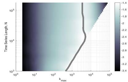
In order to explore how the HFD depends on the tuning parameter we created 100 independent time series with lengths, N, varying between 1,000 and 200,000 data points. Next, for each of these series, we compute the HFD for different values of k_max, allowing k_max to vary between k_max =2 and k_max =N/2. The idea is to produce Monte Carlo simulations from which to derive a distribution of outcomes that can be analyzed. This results in a set of HFD values as a function of the time series length, and the tuning parameter, k_max. Next, we create surface plots comparing the HFD versus the tuning parameter k_max and time series length, N. To best compare the results for various theoretical HFD from the wavelet method, we calculate an error metric, defined as, the percentage error:

 

 

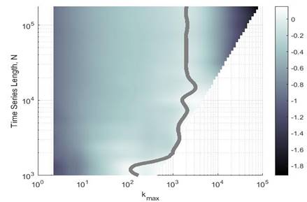
Figure 4 Surface showing the percentage error between the Higuchi algorithm and theoretical HFD=1.9. The curve of least error is shown as a thick grey line.

This error metric allows one to easily see where the Higuchi algorithm best approximates the correct HFD, and where it produces overestimates or underestimates. Figure 4, Figure 5, Figure 6, Figure 7, Figure 8 shows the surface plots for E(k_max,N) for values of HFD=1.9, 1.7, 1.5, 1.3, 1.1. The grey line overlaid in each figure shows the curves of minimum error, corresponding to the k_max tuning parameter that yields the best correspondence between the theoretical and HFD values for a given N, averaged over 100 unique time series.

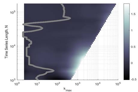
Figure 5 Surface showing the percentage error between the Higuchi algorithm and theoretical HFD=1.7. The curve of least error is shown as a thick grey line

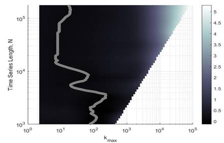
Figure 6 Surface showing the percentage error between the Higuchi algorithm and theoretical HFD=1.5. The curve of least error is shown as a thick grey line

 

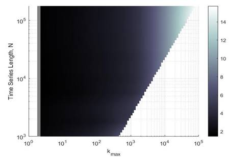
Figure 7 Surface showing the percentage error between the Higuchi algorithm and theoretical HFD=1.3. The curve of least error is shown as a thick grey line

 

Figure 8 Surface showing the percentage error between the Higuchi algorithm and theoretical HFD=1.1. The curve of least error is shown as a thick grey line

By taking a simple average of these minimum error curves of least error we are able to derive a best-fit curve using a cubic function, shown in Figure 9 as the dashed curve, for the average relationship between the time series length and the tuning parameter, for different HFD values:

 

 

 This function can be used to generate a tuning parameter estimate that can be expected to yield accurate results for the HFD, for cases where N<200,000.

Figure 9 Comparison of the average minimum error curve (solid) and the best fit cubic function (dashed).

 

4. APPLICATION TO GENETICS

We next demonstrate analysis on physical data, that of a complete genome of a bacterial organism, viz. the proteobacteria Acidovorax avenae which attacks the Cucurbitaceae family. These data are freely available from the National Center for Biotechnology Information (NCBI), which is part of the United States National Library of Medicine (NLM), a branch of the National Institutes of Health (NIH).

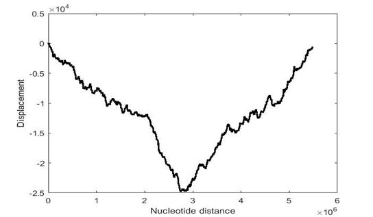
Figure 10 Acidovorax avenae complete genome represented by the Peng Abry and Sellan (1996) method.

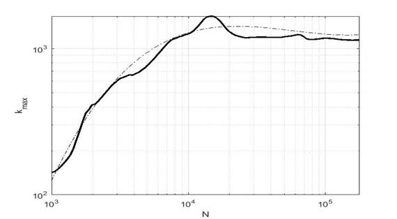
In order to analyze hidden patterns in the genome, the nucleotide sequence must be converted from a symbolic sequence, meaning A, G, C, T; to a numeric representation. The Peng method Peng et al. (1992) was followed wherein DNA is represented as a “random walk” with two parameters ruling the direction of the “walk” and the resulting displacement. Starting from the first nucleotide, every time we encounter a pyrimidine base, we move up one position. On the other hand, when a purine base is encountered in the series, we move down one position. The nucleotide distance from the first nucleotide is then plotted versus the displacement, as in Figure 10, Figure 11 shows the computed HFD against tuning parameter k_max from time series of length N=200,000 that are subsets from the original series shown in Figure 10. We took 39 non-overlapping series and computed curves for each of them. Figure 11 shows that the curves (black lines) computed from different subsets of the genome are very similar, which indicates that the fractal dimension does not vary significantly along the genome.

In each case the results show a clear plateau and an HFD<1.5, indicating a persistent time series, though with widely divergent values due to the different tuning parameter.

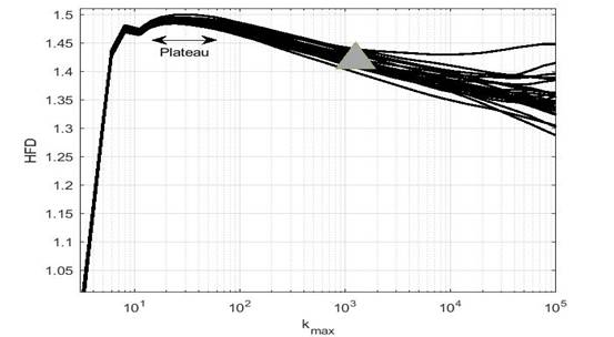
Figure 11 HFD calculated for varying length kmax between 2 and 100,000 for nonoverlapping time series of length N=200,000 from Acidovorax Avenae. The grey triangle shows where our research indicates the appropriate kmax should be situated.

 

The plateau region is shown with the arrows and, using a plateau as the measure of where to select k_max, suggests the best tuning parameter should be in the range k_max =10-50, thus yielding HFD~1.49. However, our analysis, given time series length N=200,000, recommends a value around k_max =1,000 (grey triangle) which yields HFD~1.42. This difference allows one to easily see where the Higuchi algorithm best approximates the correct HFD, and where it produces over- or underestimates.

 

5. CONCLUSIONS AND RECOMMENDATIONS

The Higuchi algorithm Higuchi (1988) is one of many widely used methods to compute fractal properties of complex nonlinear physical signals from a wide variety of research areas Esteller et al. (2001), Wanliss  and  Reynolds (2003), Mitsutake et al. (2004), Cersosimo and Wanliss (2007). Over the past decades the Higuchi algorithm has been extensively used to study pathologies in biological systems and to discriminate between healthy signals and those displaying pathologies. It is often preferred when large amounts of data are analyzed because it is stable, rapid, accurate, relatively low-cost, and excels better known linear methods for study fractal properties of a time series. However, the method requires the user to input a free tuning parameter, k_max., the selection of which influences computational efficiency of the algorithm and, more importantly, the value of the computed HFD. Thus, all the benefits of the algorithm can be negated by poor selection of the tuning parameter. Different values of k_max can produce widely divergent estimates for the HFD from the same time series, thus it is imperative to have a method for appropriately determining the best tuning.

It has been suggested (e.g., by Doyle et al. (2004) and Wajnsztejn et al. (2016)) Doyle et al. (2004), Wajnsztejn et al. (2016) that the best k_max to derive the most precise HFD should be where the calculated HFD (k_max) approaches a local maximum or asymptote, considered to be a saturation point. However, as we have demonstrated in Figure 3, it is not a given that any physical data will result in such a plateau or saturation point. This methodology can produce spurious results and can be a time consuming, iterative process.

In this paper we have explored Monte Carlo computer realisations of wavelet derived fBm time series, with known HFD. We have demonstrated that calculation of an accurate HFD depends not only on the appropriate k_max but is also dependent on time series length, N. We have calculated a relationship that determines the appropriate k_max to obtain the best HFD, given the time series length. We find that a third order polynomial will yield an appropriate k_max given the particular time series length, N. In general, persistent time series, with HFD<1.5, tended to need smaller k_max than antipersistent series.

In a future work we will extend these results to larger data sets and explore the effects from simulations of synthetic synthetic time series with known fractal properties, to see how well the method performs, and how it is influenced by the generation algorithms.

 

ACKNOWLEDGEMENTS

This work was supported by the US National Science Foundation (Grant No. AGS-2053689) and SC-INBRE.

 

REFERENCES

Abry, P. and Sellan, F., (1996). The Wavelet-Based Synthesis for Fractional Brownian Motion Proposed by F. Sellan and Y. Meyer: Remarks and Fast Implementation. Applied and Computational Harmonic Analysis, 3(4), pp.377-383. Retrieved from https://doi.org/10.1006/acha.1996.0030

Affinito, M., Carrozzi, M., Accardo, A. and Bouquet, F., (1997). Use of the fractal dimension for the analysis of electroencephalographic time series. Biological Cybernetics, 77(5), pp.339-350. Retrieved from https://doi.org/10.1007/s004220050394

Bardet, J.-M.; G. Lang, G. Oppenheim, A. Philippe, S. Stoev, M.S. Taqqu (2003), "Generators of long-range dependence processes: a survey," Theory and appli-cations of long-range dependence, Birkhäuser, 579-623.

Cersosimo, D. O., and J. A. Wanliss (2007), Initial studies of high latitude magnetic field data during different magnetospheric conditions, Earth Planets Space, 59(1), 39- 43. Retrieved from https://doi.org/10.1186/BF03352020

Doyle, T., Dugan, E., Humphries, B. and Newton, R., (2004). Discriminating between elderly and young using a fractal dimension analysis of centre of pressure. International Journal of Medical Sciences, pp.11-20. Retrieved from https://doi.org/10.7150/ijms.1.11

Esteller, R., Vachtsevanos, G., Echauz, J. and Litt, B., (2001). A comparison of waveform fractal dimension algorithms. IEEE Transactions on Circuits and Systems I: Fundamental Theory and Applications, 48(2), pp.177-183. Retrieved from https://doi.org/10.1109/81.904882

Gomolka, R., Kampusch, S., Kaniusas, E., Thürk, F., Széles, J. and Klonowski, W., (2018). Higuchi Fractal Dimension of Heart Rate Variability During Percutaneous Auricular Vagus Nerve Stimulation in Healthy and Diabetic Subjects. Frontiers in Physiology, 9. Retrieved from https://doi.org/10.3389/fphys.2018.01162

Gómez, C., Mediavilla, Á., Hornero, R., Abásolo, D. and Fernández, A., (2009). Use of the Higuchi's fractal dimension for the analysis of MEG recordings from Alzheimer's disease patients. Medical Engineering & Physics, 31(3), pp.306-313. Retrieved from https://doi.org/10.1016/j.medengphy.2008.06.010

Higuchi, T., (1988). Approach to an irregular time series on the basis of the fractal theory. Physica D: Nonlinear Phenomena, 31(2), pp.277-283. Retrieved from https://doi.org/10.1016/0167-2789(88)90081-4

Kawe, T., Shadli, S. and McNaughton, N., (2019). Higuchi's fractal dimension, but not frontal or posterior alpha asymmetry, predicts PID-5 anxiousness more than depressivity. Scientific Reports, 9(1). Retrieved from https://doi.org/10.1038/s41598-019-56229-w

Kawe, T.N.J., Shadli, S.M. & McNaughton, N. (2019) Higuchi's fractal dimension, but not frontal or posterior alpha asymmetry, predicts PID-5 anxiousness more than depressivity. Sci Rep 9, 19666. https://doi.org/10.1038/s41598-019-56229-w Retrieved from https://doi.org/10.1038/s41598-019-56229-w

Kesić, S. and Spasić, S., (2016). Application of Higuchi's fractal dimension from basic to clinical neurophysiology: A review. Computer Methods and Programs in Biomedicine, 133, pp.55-70. Retrieved from https://doi.org/10.1016/j.cmpb.2016.05.014

Khoa, T., Ha, V. and Toi, V., (2012). Higuchi Fractal Properties of Onset Epilepsy Electroencephalogram. Computational and Mathematical Methods in Medicine, 2012, pp.1-6. Retrieved from https://doi.org/10.1155/2012/461426

Klonowski, W., Olejarczyk, E. and Stepien, R., (2004). 'Epileptic seizures' in economic organism. Physica A: Statistical Mechanics and its Applications, 342(3-4), pp.701-707. Retrieved from https://doi.org/10.1016/j.physa.2004.05.045

Mandelbrot, Benoit B., and John W. Van Ness. (1968) "Fractional Brownian Motions, Fractional Noises and Applications." SIAM Review, vol. 10, no. 4, Society for Industrial and Applied Mathematics, pp. 422-37. Retrieved from https://doi.org/10.1137/1010093

Mitsutake G, Otsuka K, Oinuma S, Ferguson I, Cornélissen G, Wanliss J, Halberg F (2004) Does exposure to an artificial ULF magnetic field affect blood pressure, heart rate variability and mood? Biomed Pharmacother 58:S20-S27. Retrieved from https://doi.org/10.1016/S0753-3322(04)80004-0

Paramanathan, P. and Uthayakumar, R., (2008). Application of fractal theory in analysis of human electroencephalographic signals. Computers in Biology and Medicine, 38(3), pp.372-378. Retrieved from https://doi.org/10.1016/j.compbiomed.2007.12.004

Peng, C., Buldyrev, S., Goldberger, A., Havlin, S., Sciortino, F., Simons, M. and Stanley, H., (1992). Long-range correlations in nucleotide sequences. Nature, 356(6365), pp.168-170. Retrieved from https://doi.org/10.1038/356168a0

Shamsi, Elham, Mohammad Ali Ahmadi-Pajouh, Tirdad Seifi Ala, (2021) Higuchi fractal dimension: An efficient approach to detection of brain entrainment to theta binaural beats, Biomedical Signal Processing and Control, Volume 68, 102580. Retrieved from https://doi.org/10.1016/j.bspc.2021.102580

Wajnsztejn, R., Carvalho, T., Garner, D., Raimundo, R., Vanderlei, L., Godoy, M., Ferreira, C., Valenti, V. and Abreu, L., (2016). Higuchi fractal dimension applied to RR intervals in children with Attention Defi cit Hyperactivity Disorder. Journal of Human Growth and Development, 26(2), p.147. Retrieved from https://doi.org/10.7322/jhgd.119256

Wanliss, J. A., and M. A. Reynolds (2003), Measurement of the stochasticity of low-latitude geomagnetic temporal variations, Ann. Geophys., 21, 2025. Retrieved from https://doi.org/10.5194/angeo-21-2025-2003

Zappasodi F, Olejarczyk E, Marzetti L, Assenza G, Pizzella V, Tecchio F (2014) Fractal Dimension of EEG Activity Senses Neuronal Impairment in Acute Stroke. PLoS ONE 9(6): e100199. Retrieved from https://doi.org/10.1371/journal.pone.0100199