THE “FLU SEASONS” AND THE MISSING DATA: A MATCHED-PAIR ANALYSIS FOR THE PANDEMIC SEASON 2019_2020Vincent Kay Lo Ip *1 1 Clinical Instructor, Faculty of Medicine (Department of Family Practice), University of British Columbia, Vancouver, V6T 1Z1, Canada. |
|
||
|
|
|||
|
Received 31 July 2021 Accepted 15 August2021 Published 31 August 2021 Corresponding Author Vincent
Kay Lo Ip, vinceip@yahoo.com DOI 10.29121/granthaalayah.v9.i8.2021.4129 Funding:
This
research received no specific grant from any funding agency in the public,
commercial, or not-for-profit sectors. Copyright:
© 2021
The Author(s). This is an open access article distributed under the terms of
the Creative Commons Attribution License, which permits unrestricted use, distribution,
and reproduction in any medium, provided the original author and source are
credited.
|
ABSTRACT |
|
|
|
The
unit cell from the McNemar’s 2x2 Table denotes the week with col (1, 2) and
the Public Health Region with Row (1, 2). We calculate the standard normal
statistic (z) for A(H1), A(H3), Influenza B. Each one categorical unit is in
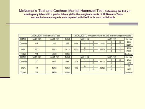
fact a pair of matched-pair data within its own partial table. The Cochran-Mantel-Haenszel Test collapses
these partial tables to summate these 2n observations in a 2x2 x n
contingency table to yield the marginal counts of the McNemar’s test. The
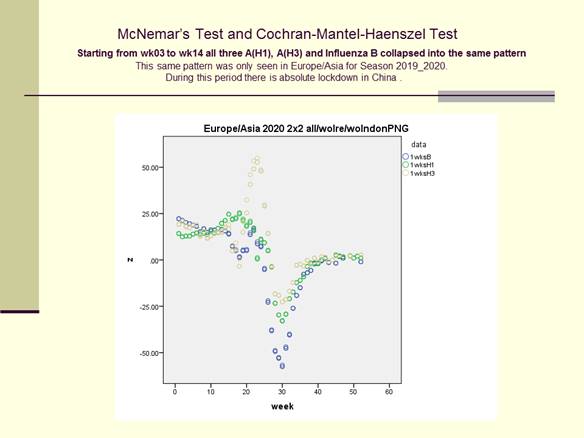
open data for Europe/Asia began this SARS-CoV2 pandemic, from week 3 to week
14, with the normal statistic (z) entering into an identical collapse
mode. These all assumed the same “V”
curve as the general collapse pattern and they rippled together without
overlapping. During this period China applied mandatory lockdown and they
mandated masks. We should strive to be more evidence-based so that we can
convince more of the general public to accept the public health measures to
survive. Background:
The matched-pair analysis does not compare between viruses or the
different laboratory practices. Each virus among n is match-paired with
itself in the two responses of its own partial table. The
Cochran-Mantel-Haenszel Test summates all these partial tables to arrive at
the same marginal counts of the McNemar’s Test. This test statistic is
likewise used for the Rasch model and for the Transmission Dysequilibrium
Test. Methods
And Results: We used col (1, 2) =1wk for N_America, Europe/Asia
and forS_America/Africa/Australia/New_Zealand. For Canada Row1/Row2 was (BC-
Manitoba)/ (Ontario-Atlantic). For the US Row1/Row2 was Regions (7-10)/ (1-6).
We performed simultaneous Proportional Odds Comparison of Margins (4x4
Table). We sequentially deleted Regions 1, 10, (9-10), (8-10), (1-4) and (1-
5) to define the effects of the missing data. And we surveyed for ILI
pneumonias in Hong Kong for matched-pair regression. A(H1) and A(H3)
surged/resurged with condition numbers (multicollinearity)=<(φ)=(eigenvaluemax/eigenvaluemin)
=(λmax/λmin) At above 2,962 the regression coefficients diverged in
opposite directions. Conclusions:We
define the the Influenza Season since 2019_2020 mathematically with the
McNemar’s Test using the Laboratories’ real-time observations from the
Americas, Europe/Asia, Afri We
define ca and Australia/New_Zealand. These real-time sequential frames from
the weekly updated data show that z=(n12-n21)/(n12+n21)
^0.5 holds for the normal and for the approximate standardized test
statistics. |
|
||
|
Keywords: Analysis,
Pandemic, Season, Matched |
|
||
1. INRODUCTION
The SARS-CoV-1 epidemic in 2002-2003 provided the background of this study when this started in Hong Kong. The first evidence of the epidemic in 2003 was actually noticeable from November 2002 when the SARS-CoV-1 was sequenced in April 2003 Peiris et al. (2004). China was able to limit that epidemic to 5329 confirmed clinical cases with 349 deaths in 2003 WHO. (2003). And Hong Kong quashed the epidemic with only 1750 confirmed cases and 299 mortalities. (World Health Organization (WHO), 2020). As at July 2020 these numbers for SARS-CoV-2 had surpassed 14 million globally with over 600,000 deaths. The WHO consensus since May 2003 3 is still relevant. A textbook on mathematical statistics defines Complete Sufficient Statistics and the search for minimum variance estimators. HOGG et al. (2013)
This “Current” situation as changed from 2003 to 2020. WHO (2020), Drosten et al. (2003), Marra et al. (2003), Roy and Milton (2004).
The opportunistic airborne transmission of SARS had finally got past the direct person-to-person small-particle aerosols transmission to cause this SARS-CoV-2 pandemic in 2020. The Avian Influenza (H5N1) cannot yet spread by small-particle aerosols Beigel et al. (2005). This global person-to-person transmission of SARS-CoV-2 is efficient by airborne and droplet routes Meselson (2020) . New methods of sampling Cheng et al. (2019) are attempting to define the infecting dose or to define super-spreaders. This direct transmission is controllable or reducible by social distancing and masks. Chu et al. (2020) The efficiency that the virus transmits Panel EA et al. (2020) renders previous worldwide stockpiling strategies Balicer et al. (2005) unable to provide the early needs of personalized protective equipment, hospital beds and ventilators. Castro et al. (2020).
The Survey from 2004 to 2009
The aim in 2004 was to find the “sufficient statistic”. Simple Random Sampling Scheaffer (2007) was performed from 2004 to 2009. Out of every 100 questionnaires that were sent out every week, 15 to 20 copies returned. The parameters were “fever”, “cough”, “difficulty breathing”, “pneumonia”, “contact with ILI”, “bacterial infections”, and “hospitals”. We used Proc Freq and Proc Genmod in 2004 and we switched to Proc Glimmix in 2007. Proc Freq and Proc Genmod suggested that the parameters “pneumonia” and “contact with ILI” to be likely candidates to be the “sufficient statistic”. Proc Glimmix confirmed that these two parameters showed remarkable convergence on iterative computations. Kay (2014).
The Binomial Distribution
Each coin is unique, where each and every coin-flipping is also unique, and there is a unique subject-specific effect HOGG (2013) every time. In fact, each and every virus has a behavior that must be unique to itself for that moment in time. Assuming that we are inside the contingency table of this one single virus proceeding from one moment to the next, we have n=2 independent trials, and the three different possibilities of one win, two win or no win for Y:
![]()
![]()
The Questionnaire

In terms of the Cochran Mantel Haenszel Test and the McNemar’s Test, and if each of the n 2x2 contingency table is truly independent, it would have a binomial distribution as in the following:
Let Y denote the number of successes. The probability of success y=2, with n=2 trials, for cell row 1 and column 1.
The probability of failure y=0, with n=2 trials, for cell row 2 and column 2,
![]()
![]()
The probability of success y=1 with n=2 trials, for cell row 1 and column 2
And for cell row 2 and column 1
![]()
![]()
The Serial conditional probability function
The situation of the single virus within its own partial table at any moment in time and facing its own unique choices can be represented as a continuous serial conditional probability function where the uncertainties in the numerator and the denominator are equal at any one instantaneous moment and they cancel each other out. HOGG (2013)

According to the prevalent concept of the “missing data” at the time, our findings relevant to the parameter’s “pneumonia” and the “history of contact” with influenza-like-illness were therefore most surprising.
Pneumonia and contact with ILI
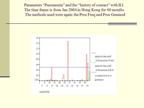
This is the Graph for Parameters “Pneumonia”. The graph for the history of “contact” with ILI is not showed as it had a much more reduced range of “ɑ<0.05 significance” for the “ß coefficients”. The time frame for both is from January 2004 in Hong Kong for a period of 60 months. The methods that were used were the Proc Freq and Proc Genmod. This graph monitored the “ɑ<0.05 significance” of the “ß coefficients” for the categorical counts of the parameter “pneumonia”, reporting Wald and LR statistics as described for the method. The blue line is for the accepted significance level of ɑ<0.05. Red is for the Wald stat and green is for the LR stat. It is clear that from this graph that, with either the Wald or the LR statics, during most of the 60 months during the survey, the significance level of the ß coefficients reached the accepted level of ɑ<0.05. This meant that most of the parameters of “pneumonia” obtained during the survey were significant for computation in the ordinary mathematical sense. It is important to note that, while most of the “pneumonia” parameters were significant enough to reach the ɑ<0.05 significance level, there were three months out of a total of 60 months, where the ɑ significance level did break over to above and beyond the accepted ɑ<0.05 significant level.
2. METHODS
The MATCHED-PAIR Relationship -- the Null Hypothesis
The null hypothesis is that the moment to moment (i.e.,
real-time) changing or non-changing westerly (or northerly) winds have no
relation with the distribution of the virus isolations within the geographic
areas. This becomes a test for the matched-pair relationship. Agresti (2006) The streamline flow or
the turbulence Haines and Malanotte-Rizzoli (1991) has no relation to the
timing and the geographic location of the actual viral landings. From 2011 we
used the loglinear model ML estimate ![]() to show the
estimated probability that response on geographic location is x categories
higher than the response on time equals exp(
to show the
estimated probability that response on geographic location is x categories
higher than the response on time equals exp(![]() x) times the reverse probability. From 2010_2011 we
used the logit model
x) times the reverse probability. From 2010_2011 we
used the logit model ![]() to denote a
parameter for each subject the odds that the row response falls in category j
or below (instead of above category j) are exp(β) times the odds for the
column response. The cross-classification in the above 2x2 Table (McNemar’s
Test) where n=3638 actually presents 2n responses for the results of two
surveys, those of the first survey in the horizontal row marginal counts and
those of the second survey in the vertical column marginal counts. The
Cochran-Mantel-Haenszel Tests on the above right present these same data
differently as n=3638 separate 2x2 partial tables, one partial table for the
two matched responses from each virus. Each 2x2 partial table has one column
for each possible outcome, and the results of the first survey in row 1, and
the results of the second survey in row 2. And collapsing the 2x2 x n
contingency table for USA and Canada yields the marginal counts of the
McNemar’s tests.
to denote a
parameter for each subject the odds that the row response falls in category j
or below (instead of above category j) are exp(β) times the odds for the
column response. The cross-classification in the above 2x2 Table (McNemar’s
Test) where n=3638 actually presents 2n responses for the results of two
surveys, those of the first survey in the horizontal row marginal counts and
those of the second survey in the vertical column marginal counts. The
Cochran-Mantel-Haenszel Tests on the above right present these same data
differently as n=3638 separate 2x2 partial tables, one partial table for the
two matched responses from each virus. Each 2x2 partial table has one column
for each possible outcome, and the results of the first survey in row 1, and
the results of the second survey in row 2. And collapsing the 2x2 x n
contingency table for USA and Canada yields the marginal counts of the
McNemar’s tests.
The Missing Data
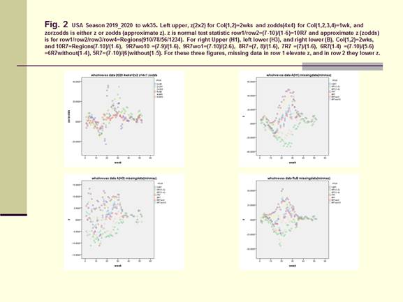
The 10-Region who/nrevss regional map contained the full version of the official data Regions. The 9-Region who/nrevss regional map showed how the observations could be missing or misplaced. The official 10-Region map carried the numbers (1-10) of the data Regions in bold and these numbers (together with their data) corresponded to the respective Regions in the 9-Region map, where Region 10 and its data were missing. We sequentially defined Regions 1, 10, (9-10), (8-10), (1-4) and (1-5) as further missing data and we presented these comparisons in the extreme conditions of Figure 2.
For weekly real-time computations we needed to define the entity of the interim missing data at the beginning of the week and which would be updated in the subsequent days before the end of the week.
3. RESULTS
The McNemar’s Test and the Wald test (Proportional
Odds Model)
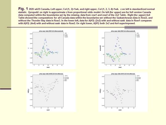
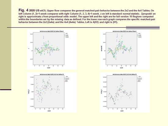
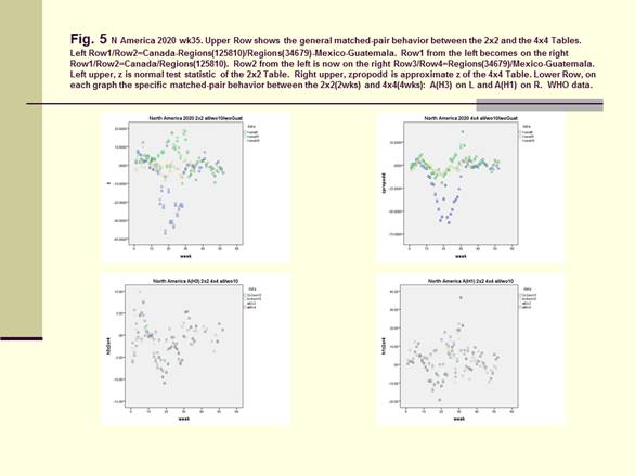
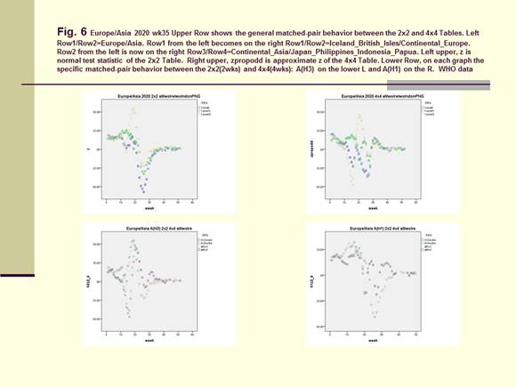
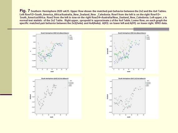
On Figure 1 for Canada, Figure 4 and Figure 8 for the US, Figure 5 for North America, Figure 6 for Europe/Asia, and Figure 7 for the Southern Hemisphere, we tested the matched-pair model generally with the standardized normal test statistic z of the McNemar’s Test on the upper left and compared this with the approximate z based on the Proportional Odds Model on the upper right. On the lower row within each graph, we superimposed the 2x2 (2wk) and 4x4 (4wks) Tables to compare for A(H3) on the lower left and A(H1) on the lower right.
|
|
|
Figure 1 The McNemar’s Test and the Wald Test for Virus
Isolation Data |
For Figure 2, the left upper diagram showed the full version of the official data (2x24wks) Row1/Row2= (7-10)/ (1-6) =10R7 and (4x4 4wks) Row1/Row2/Row3/Row4 =Regions (910/78/56/1-4). The right upper (AH1), left lower (AH3) and right lower (B) diagrams showed the effects of the missing data (min and max) from both sides of Row1 or Row2 in the 2x2 Table Column (1, 2) =2 wks. The three center-most curves in each of these three diagrams were represented by 10R7=Row1/Row2= (7-10)/ (1-6), 9R7 without 10=Row1/Row2 = (7-9)/ (1-6) and 9R7 without 1=Row1/Row2= (7-10)/ (2-6). The upper boundaries were represented by 8R7=Row1/Row2= (7-8)/ (1-6) and 7R7=Row1/Row2= (7)/ (1-6. And the lower boundaries were by 6R7= (7-10)/ (5-6) without regions (1-4) and 5R7= (7-10)/ (6) without regions (1-5). With these missing data defined for Row1 the entire curves for 8R7=Row1/Row2= (7-8)/ (1-6) and for 7R7=Row1/Row2= (7)/ (1-6) moved upwards along the y-axis. The opposite occurred for Row1/Row2=6R7= (7-10)/ (5-6) without regions (1-4) and for Row1/Row2=5R7= (7-10)/ (6) without regions (1-5). These moved downwards along the y-axis.
|
|
|
Figure 2 The Missing Data (minimized and maximized) |
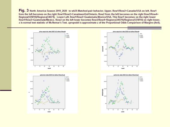
In Figure 3 we computed the full data from Canada, USA, as Row1/Row2=North/South =Canada/USA =BC-Atlantic/Regions (1-10) and the full data from Mexico, Guatemala and USA as Row1/Row2= South/North=Mexico-Guatemala/USA. For Canada/USA we computed these to be within the boundaries formed with Row1=BC-Atlantic Provinces without the Thunder Bay data and with Row2=Regions (1-9) without region 10. On the right upper graph, the data were Row1/Row2/Row3/Row4=CanadawoOnt/Ontario/Region (125810)/Region (34679). Incomparing the 2x2 Table with the 4x4 Table it was found that the original boundary between Row1/Row2 should be kept intact as the boundary between Row2/Row3. For the Same reason, the 2x2 Table for Mexcio-Guatemala/USA was compared with Row1/Row2/Row3/Row4=Guatemala/Mexico/Regions (34679)/Regions (125810).
|
|
|
Figure 3 Row1/Row2=Canada/USA and
Row1/Row2=Mexico-Guatemala/USA |
Figure 4 and Figure 5. The McNemar’s Test and the Proportional Odds Model.
The full version of the data represented by 10R7=Row1/Row2= (7-10)/ (1-6) were computed to be within the two boundaries set between 9R7 (without 10) = Row1/Row2 = (7-9)/ (1-6) and 9R7 (without 1) =Row1/Row2 = (7-10)/ (2-6).
|
|
|
Figure 4 The
McNemar’s Test and the Proportional Odds Model |
From a higher vantage point, we computed the whole of North America with row1/row2=Canada-Regions (125810)/Regions (34679)-Mexico-Guatemala and with row1/row2/row3/row4=Canada/Regions (125810)/Regions (34679)/Mexico-Guatemala in Figure 5.
|
|
|
Figure 5 The
McNemar’s Test and the Proportional Odds Model. |
|
|
|
Figure 6 WHO data for Europe/Asia |
|
|
|
Figure 7 WHO data for the Southern
Hemisphere |
The full version of the data represented by 10R7=Row1/Row2= (7-10)/ (1-6) were computed to be within the two boundaries set between 9R7(without 10) = Row1/Row2 = (7-9)/ (1-6) and 9R7(without 1) =Row1/Row2 = (7-10)/ (2-6).
|
|
|
Figure 8 The McNemar’s Test and the
Proportional Odds Model as it applies to Influenza B and the Victoria and
Yamagata lineages |
Mathematical Model for Regression Analysis
The model is an example of mixed model, containing the
random effect ![]() i (intercept) and the fixed effect (
i (intercept) and the fixed effect (![]() ).
For PROC GLIMMIX, the outcome ‘1’ is ‘successes and outcome ‘0’ is ‘failure’
for the response of pneumonia in the univariate 2-stacked data format. Let
ψi denote the probability of a
success for subject i’s response:
).
For PROC GLIMMIX, the outcome ‘1’ is ‘successes and outcome ‘0’ is ‘failure’
for the response of pneumonia in the univariate 2-stacked data format. Let
ψi denote the probability of a
success for subject i’s response:
Logit(ψi) = i + ![]() 1[A(H1N1)]
+
1[A(H1N1)]
+ ![]() 2[A(H3N2)]
+
2[A(H3N2)]
+ ![]() 3[B]
+
3[B]
+ ![]() 4[C] +
4[C] +
![]() 5[PFLU] +
5[PFLU] + ![]() 6[MYCO]
+
6[MYCO]
+ ![]() 7[RSV]
+
7[RSV]
+ ![]() 8[contact*estimator] Equation 2
8[contact*estimator] Equation 2
![]() i the
intercept representing an unobserved sample from a probability distribution,
presumed to be normal distribution with unknown mean and standard deviation.
i the
intercept representing an unobserved sample from a probability distribution,
presumed to be normal distribution with unknown mean and standard deviation.
Response (event= ‘1’) denotes the probability of a success for subject i’s response;
![]() 1,
1, ![]() 2,
2, ![]() 3,
…… and
3,
…… and ![]() 8
are coefficients for weekly respiratory virus isolations;
8
are coefficients for weekly respiratory virus isolations;
Estimator = H1N1, H3N2, B, C, PFLU, MYCO, rsvp, virus*virus.
fh1, fh3 and fb is H1N1, H3N2 or b expressed as fraction of samples;
contact number of patients per week who develop ILI’s after contact with
other patients who had ILI’s
We re-computed our data with PROC GLIMMIX from December 2004 onwards. We performed univariate regression analysis for pneumonia using Response(event=1), ‘1’ being success and ‘0’ being failure for pneumonia. The two response parameters of ‘pneumonia’ (binary) and ‘contact’ (Poisson) were stacked in the 2-tiered univariate format Edition (2009). We computed the random (αi) effects and the fixed (β) effects for the different components of Virus Isolation Data 2004-2009 in accordance with our model, and Probability=pi=exp(αi+β)/(1+exp(αi+β) for “Response(event=1)”, this being the subject-specific effects from the ith questionnaire and ith partial table of the McNemar’s Test. Note: Model is modified from PROC GLIMMIX documentation (STAT 9.2 User’s Guide_ The GLIMMIX Procedure (Book Excerpt) - statugglmmix.pdf, n.d.). The McNemar’s Test and matched-pair data provided the model for this survey for matched-pair data, ‘1’= success and ‘0’=failure for ILI pneumonia. PROC GLIMMIX computed the random(αi) and fixed(β) effects for A(H3N2) and A(H1N1). We defined
pi=Probability (event= ‘1’) =exp(αi+β)/(1+exp(αi+β))
as the subject-specific-effects from the ith questionnaire and partial table.
4. DISCUSSIONS
The estimations of the Basic Reproduction Numbers Alimohamadi et al. (2020), Mills et al. (2004) differ widely for this Covid-19 pandemic. These airborne transmissions Tellier (2006), Stadnytskyi et al. (2020) are efficient to transmit between persons. The SIRC/SIR model Casagrandi et al. (2006) provides the scientific basis for “flattening or crushing the curve”. We present the best available collateral evidence in the form the simultaneous isolations for the influenza viruses (A(H1), A(H3) and Influenza B), when the lockdown was applied to every person in Wuhan (Figure 6) to stop the transmissions of Covid-19. In those other parts of the world, lockdown was either mandatory or voluntary, and the surgical mask was also mandatory or voluntary. The final practical means of crushing the curve comes to these different forms of social distancing with or without the mandating of the surgical mask. Lewnard (2020). The McNemar’s statistic provides this evidence-based perspective on the collateral means (and ends) to the flattening of this curve. This collateral evidence focused on the surgical face-mask when this helps to cuts the transmissions of both the small-particle aerosols and the large droplets Anfinrud et al. (2020)between persons. In Figure 6 the collapse pattern for influenza can be seen both in the 2wk (week-to-week) graph and in the 4week (2week-to-2week) graph.
|
|
Acknowledgmnents: To the frontline medical workers and doctors of Hong Kong and globally elsewhere.
REFERENCES
Agresti A (2006). An Introduction to Categorical Data Analysis: Second Edition. Retrieved from https://doi.org/10.1002/0470114754
Alimohamadi Y, Taghdir M, Sepandi M. (2020) Estimate of the Basic Reproduction Number for COVID-19: A Systematic Review and Meta-analysis. J Prev Med Public Health. Retrieved from https://doi.org/10.3961/jpmph.20.076
Anfinrud P, Stadnytskyi V, Bax CE, Bax A. (2020) Visualizing speech-generated oral fluid droplets with laser light scattering. N Engl J Med. Retrieved from https://doi.org/10.1056/NEJMc2007800
Balicer RD, Huerta M, Davidovitch N, Grotto I. (2005) Cost-benefit of stockpiling drugs for influenza pandemic. Emerg Infect Dis. Retrieved from https://doi.org/10.3201/eid1108.041156
Beigel JH, Farrar J, Han AM, et al. (2005) Avian influenza A (H5N1) infection in humans. N Engl J Med;353(13) :1374-1385. Retrieved from https://doi.org/10.1056/NEJMra052211
Casagrandi R, Bolzoni L, Levin SA, Andreasen V. (2006) The SIRC model and influenza A. Math Biosci.. Retrieved from https://doi.org/10.1016/j.mbs.2005.12.029
Castro MC, Carvalho LR de, Chin T, et al. (2020) Demand for Hospitalization Services for COVID-19 Patients in Brazil. Retrieved from https://doi.org/10.1101/2020.03.30.20047662
Cheng VCC, Wong SC, Chan VWM, et al. (2019) Air and environmental sampling for SARS-CoV-2 around hospitalized patients with coronavirus disease (COVID-19). Infect Control Hosp Epidemiol. 2020. Retrieved from https://doi.org/10.1017/ice.2020.282
Chu DK, Akl EA, Duda S, et al. (2020) Physical distancing, face masks, and eye protection to prevent person-to-person transmission of SARS-CoV-2 and COVID-19: a systematic review and meta-analysis. Lancet. Retrieved from https://doi.org/10.1016/S0140-6736(20)31142-9
Drosten C, Günther S, Preiser W, et al. (2003) Identification of a novel coronavirus in patients with severe acute respiratory syndrome. N Engl J Med. Retrieved from https://doi.org/10.1056/NEJMoa030747
Edition S. (2009) User ' s Guide. SAS/STAT® 92 User's Guid Second Ed.
HOGG R V, MCKEAN JW, CRAIG AT (2013). Introduction to Mathematical Statistics.
Haines K, Malanotte-Rizzoli P. (1991) Isolated anomalies in westerly jet streams: a unified approach. J Atmos Sci. Retrieved from https://doi.org/10.1175/1520-0469(1991)048<0510:IAIWJS>2.0.CO;2
Health WHO, Programme E, Panel EA, et al. (2020) Transmission of SARS-CoV-2 : implications for infection prevention precautions.(July):1-10.
Kay V. (2014) The "Flu Seasons" and the Missing Data: A Matched-Pair Analysis Northern and Southern Hemispheres 2013-2014 and Hong Kong, China 2004-2009. J Hum Virol Retrovirology ;1(4):1-10. Retrieved from https://doi.org/10.15406/jhvrv.2014.01.00023
Lewnard JA, Lo NC. (2020) Scientific and ethical basis for social-distancing interventions against COVID-19. Lancet Infect Dis. Retrieved from https://doi.org/10.1016/S1473-3099(20)30190-0
Marra MA, Jones SJM, Astell CR, et al. (2003) The genome sequence of the SARS-associated coronavirus. Science (80). Retrieved from https://doi.org/10.1126/science.1085953
Meselson M. (2020) Droplets and aerosols in the transmission of SARS-CoV-2. N Engl J Med. Retrieved from https://doi.org/10.1056/NEJMc2009324
Mills CE, Robins JM, Lipsitch M. (2004) Transmissibility of 1918 pandemic influenza. Nature. Retrieved from https://doi.org/10.1038/nature03063
Peiris JSM, Guan Y, Yuen KY. (2004) Severe acute respiratory syndrome. Nat Med. Retrieved from https://doi.org/10.1038/nm1143
Roy CJ, Milton DK. (2004) Airborne Transmission of Communicable Infection - The Elusive Pathway. N Engl J Med. Retrieved from https://doi.org/10.1056/NEJMp048051
STAT 9.2 User's Guide_ The GLIMMIX Procedure (Book Excerpt) - statugglmmix.pdf.
Scheaffer RL, Mendenhall III W, Ott RL. (2007) Elementary Survey Sampling.
Stadnytskyi V, Bax CE, Bax A, Anfinrud P. (2020) The airborne lifetime of small speech droplets and their potential importance in SARS-CoV-2 transmission. Proc Natl Acad Sci U S A.. Retrieved from https://doi.org/10.1073/pnas.2006874117
Tellier R. (2006) Review of aerosol transmission of influenza A virus. Emerg Infect Dis. Retrieved from https://doi.org/10.3201/eid1211.060426
WHO, (2020) Aylward, Bruce (WHO); Liang W (PRC). Report of the WHO-China Joint Mission on Coronavirus Disease 2019 (COVID-19).
WHO. (2003) Consensus document on the epidemiology of severe acute respiratory syndrome (SARS). World Health:1-47. Retrieved from https://doi.org/10.1007/s10856-009-3765-6
World Health Organization (WHO) (2003). Emergencies preparedness, response Summary of probable SARS cases with onset of illness from 1 November 2002 to 31 July 2003. 2020;9(July):2003-2005.
 This work is licensed under a: Creative Commons Attribution 4.0 International License
© Granthaalayah 2014-2021. All Rights Reserved.