Article Citation: O.H. Aliyu, and A.A Salihu. (2021). NON-LINEAR FINITE ELEMENT ANALYSIS OF DYNAMIC PROBLEMS. International Journal of Engineering Technologies and Management Research, 8(4), 79-93. https://doi.org/10.29121/ijetmr.v8.i4.2021.926

 

Published Date: 29 April 2021

 

Keywords:

Nonlinear Analysis

Material Non-Linearity

Geometric Non-Linearity

Linearization

Joint Rotation
ABSTRACT

A formulation of the displacement based finite element method as well as the incremental analysis procedure which is considered suitable for analysis of non-linear dynamic problems is presented. The presented framework is used to investigate the influence of joint rotation on the failure of steel beam subject to high-speed impact load. The results from the non-linear numerical simulation are compared with those obtained from an analytical technique.

Method: The non-linear Full Newton Raphson method was used for the simulation and results obtained were verified analytically using the energy momentum balance technique.

Results: The beam suffered an initial vertical downward deflection of 27.7mm from the impactor load as well as a joint rotation of 2⁰.

Findings: From the results obtained the beam was considered to have failed due to excessive rotation. Similarly, from the comparism made between the analytical and non-linear numerical simulation results, it was concluded that the full Newton Raphson technique gave accurate results in simulating the dynamic problem which was achieved at an affordable cost.

1.     INTRODUCTION

 

The analysis of damage in materials and structures subjected to dynamic loadings such as blast, impacts, earthquake, fire and so on, is considered crucial. For such dynamic loadings (generally involving plasticity and damage), the complete displacement form of finite element analysis is mostly used especially where material non-linearity is considered. This displacement version of finite element analysis is generally easier to implement particularly for complicated non-linear constitutive relations. It also offers the advantage of properly modelling the element behaviour (Stein, 1993; De Borst et al, 2012; Aliyu, 2019).

In this paper, the non-linear finite element method is applied to the material’s non-linear problem involving a steel beam subjected to impact loads. The method was used to study the deformation and rotation of the beam to the dynamic impact loads. The accuracy of the non-linear finite element simulation results, in assessing deformation was compared to those obtained from comparable hand calculations and has proved to be quite satisfactory.

 

 

 

 

2.      FORMULATION OF THE NON-LINEAR FINITE ELEMENT METHOD

 

2.1. FORMULATION OF THE WEAK FORM OF THE EQUATION OF MOTION

 

In arriving at the non-linear finite element expression for solving dynamic problems we begin by adopting the concept of equilibrium and virtual work in obtaining an expression for the equation of motion where the idea of linear momentum balance is assumed.

First, we consider the balance of momentum between the body V as well as its boundary S with the stress vector t and gravity acceleration put together in the vector g resulting in the linear momentum balance expressed as:

 

 

The above expression momentum balance can be further adjusted to give the expression as shown in eqn. (1.1)

 

 

Now applying the Gauss divergence theorem to the first expression in eqn. (1.1) converts it from a surface integral to a volume integral expressed in eqn. (1.2) after rearrangement.

 

 

The integrand in eqn. (1.2) must be equal to zero which gives the local form of the balance of linear momentum also called the equilibrium equation or the equation of motion in the strong form which is thus expressed in eqn. (1.3) (Laursen, 2003; De Borst et al, 2012):

 

 

Where:      

 Is the mass density

Is the differentiation of displacement with respect to time

 Is the matrix format of the gradient vector operator at the deformed configuration

 

 

 

.

 

 

 

By inserting eqn. (2) in eqn.(1) the equation of motion can be rewritten in matrix form as

 

 

In adopting the principles of virtual work, equation (3) is further transformed into a weak form as given in eqn. (5) after applying the divergent theory to eqn. (4) which was arrived at by multiplying by a virtual displacement  to eqn. (3) and integrating over the domain V (which is the current configuration) (Kim 2018; De Borst et al, 2012).

 

 

It can therefore be seen from equation 5 that the weak form is a balance between the internal virtual work and the external virtual work (i.e., the body forces and surface traction) (Kim, 2018). It is important to stress that, in the arriving at the expression in equation 5, no guess was made with respect to the material behaviour or size of the spatial displacement gradients. Hence, equation 5 can be used for both linear and non-linear behaviours. 

 

2.2. DISCRETIZATION; FINITE ELEMENT FORMULATION

 

In this section the displacement based finite element formulations are discussed.  This section starts with finding the approximate solution to the above weak form of equation of motion. For this method, the element nodal displacements   having components (,,) is regarded as the unknown in the assumed continuous displacement field (u) given in eqn. (6) for each finite element used in the spatial finite element discretization.

 

Where:

 is the shape or interpolation polynomial function expressed in natural dimensionless coordinates .

In order to evaluate the displacement field, for points within the elements which are not key points (i.e., not nodal points) eqn. (7) is adopted.

 

 

The element strain, given in terms of the derivative of the displacement field (u) is obtained from eqn. (7.1) (Laursen, 2003; De Borst et al, 2012; Hartmann, 2005)

 

                                                                           Lu  

 

It should be noted that the measure of strain tensor to be used in equation 7.1 has not been specified as the equation is expected to be used in both linear and non-linear regime as mentioned above in the formulation of the weak form of the equation of motion.

 

                                                                 

 

Where:

  gives the matrix of shape function for the 3d element

is the matrix vector of the displacement degree of freedom at the nodal points of each element in the finite element mesh.

While eqn. (9) maps the element displacement vector ( ) to the global displacement vector () using the incidence matrix ( ) (De Borst et al, 2012; Hartmann, 2005)

 

 

Substituting eqns. (7) and (9) into the weak form of equation (5) gives equation of motion for the entire finite element mesh expressed as shown in eqn. (10):

 

 

Solution of equation (10) for every virtual displacement () leads to a semi-discrete balance of momentum as expressed in eqn. (11) since the discretisation here pertains only to the spatial domain and not to the time domain (De Borst et al, 2012).

 

Where:

 Is the mass matrix

 

 

 Is the external force vector

 

 

 

 Is the internal force vector

 

 

 

Is the matrix that relates the strains within the finite elements to the nodal displacements expressed as the derivative of the shape function as given in eqn. (16) (The above definition for  holds for a linear expression, for a non-linear expression, it relates the variations of strains within the finite elements to the variations of the nodal displacement) (De Borst et al, 2012; Hartmann, 2005).

 

 

The shape function  has been expressed in dimensionless isoparametric natural coordinates in order to facilitate the numerical integration of the integrals where complex non-linear structural geometries as well as material non-linearities are involved (Stein, 1993; De Borst et al, 2012; Seshu, 2012).

 Isoparametric finite elements have been used for this formulation as the same shape function given in eqn. (17) has been used for both the geometrical and displacement interpolations.

 

 

Where: equation 17 is a linear relationship in isoparametic coordinates

are the shape functions

gives all the finite element nodal points

 are the nodal point displacements

 

2.2.1. LINEARIZATION

 

Nonlinear problems almost always result in nonlinear equations which have to be solved by first linearizing the nonlinear equations and then solving the linearized equations (i.e., getting the roots of the equation) iteratively using appropriate techniques (such as: Newton Rahpson technique, Arc length or path following method as well as the line search method) until the solution to the problem is obtained. On the other hand, the linearized equations can be solved directly using some other solution technique, which does not require iterative solution method.  The focus here is on iterative solution technique using the Newton Rahpson method where correct linearization of the nonlinear equation is key to getting an accurate solution by ensuring quadratic convergence.

 

2.3. INCREMENTAL ANALYSIS

 

For the non-linear analysis, the application of external load as in eqn. (11) is done incrementally, that is, in load steps as opposed to the sudden application of the full external load in one single load step (Stein, 1993). This is because the set of algebraic equations which evolves as a result of finding the solution to the finite elements is non-linear. Similarly, the application of load incrementally enables the proper convergence of the solution (De Borst et al 2012; Kim, 2018). This is the preferred approach especially for rate dependent materials where the stress depends upon the history of deformation (or straining) (Laursen, 2003; Ayoub & Filippou 1998; Kim, 2018). For such materials, accurate modelling of behaviour under loading can only be achieved if the history of straining is carefully followed. Hence, justifying the need for incremental load application which allows for small strain increments to be achieved, enabling the straining path to be carefully followed (Laursen, 2003). Hence, for this incremental load process, equation (11) becomes reduced to:

 

Where the inertial term is omitted.

For loading to be applied sequentially, the time parameter is used to order the sequence of loading (that is the load steps or increments) (Laursen, 2003). In line with this preceding statement, the unknown stress vector   is additively decomposed as expressed in eqn. (19)

 

 

Where:

Is when the stress component is known at the time t

 Is the unknown component of the stress increment

Using eqn. (19) in eqn. (18) above with eqn. (15) gives the expression in eqn. (20)

 

 

Where, the second term in the right side of eqn. (20) above represents the internal virtual work done. Since the volume of the element () where the integral in eqn. (20) applies is not known at the time, it can be solved by mapping it back to reference configuration (i.e., the Lagrangian configuration).

 

 

Equation (20) above can equally be written as in eqn. (21) since we are concerned here with linearizing the source of geometric non-linearity (i.e., the nodal displacements) and removing the dependence on it. Equation (21.1) is the unbalanced force at the nodes:

 

 

 

Where:

 is the internal force vector evaluated at the time t where  (Wang & Hsu, 2001; De Brost et al.2012)

Because of the non-linear nature of equation (21) its solution necessitates the need for an iterative approach. To achieve this, the non-linear equation must first be linearised and then solved iteratively. The most frequently used iterative method is the Newton-Raphson method which entails working out the residual as well as the tangent stiffness matrix for each iteration from the weak form (Wang & Hsu, 2001; Ayoub & Filippou 1998; Hartmann, 2005; Tsavadaris, & Mello, 2012; Barth, & Wu, 2006; Kim 2018). As mentioned before, the solution of non-linear equations, entails iterative linearization of the governing equations.  For example, linearizing the dependence of the stress increment to the displacement increment expressed as shown in eqn. (23) remembering of course that no guess has been made with respect to the material behaviour (i.e., the stress and strain measure) as mentioned earlier on page 4 (Laursen, 2003; De Brost et al.2012). The increase in stress is expressed as in eqn. (22) which is then linearized as expressed in eqn. (23)

 

 

 

With

Where:

 Is referred to as the material tangential stiffness matrix

 Equation (23) can therefore be rewritten as:

 

 

(Laursen, 2003; De Brost et al.2012; Kim, 2018).

With the quasi-static loading, eqn. (18) written as:

 

 

This can be further expressed as in eqn. (27)

 

Where:

 

  is the work conjugate strain measure

Remembering of course that no assumptions have been made here, with respect to the nature of the stress or strain measures.

Considering equations (7), (9), (16) and (25), in the above non-linear expression of eqn. (21) leads to the linearized equation for finite load increment which is given in eqn. (28)

 

With the loading steps, ranging from time  to time  The material tangential stiffness matrix K is equally expressed as in eqn. (28.1). Since the increase in nodal displacement does not rely on the spatial coordinates, it can also be placed outside of the integration.

 

 

Hence equation (28) can be rewritten as:

 

 

orwith the external force vector additively decomposed and expressed as in eqn. (29.1)

 

 

These linearizations of the load steps as given in eqn. (29) as well as the linearization of the governing stress-strain equation given in (25) tend to move the solution away from the actual equilibrium solution (especially when the initial estimate of the assumed displacement is too far from the actual solution). This divergence can be reduced by incorporating equilibrium iterations inside each loading step. With this incremental-iterative solution technique, the initial displacement estimates are derived as follows:

 

Where:

 

The subscript 0 signifies the beginning steps while subscript 1 refers to the first iteration. Hence, the beginning internal force is expressed as:

 

 

 

Where:

is the determinant of the Jacobian used in the transformation between the natural isoparametric coordinates () and the corresponding Cartesian coordinates () (see figure 1)?

 

Figure 1: shows the concept of transformation between isoparametric and Cartesian coordinates adapted from Stein 1993.

 

The stress  after the beginning steps (that is the stress in the first iteration) is then derived from eqn. (33)

 

 

As initially mentioned, there is usually a divergence of the actual true solution from the equilibrium solution which is why the original force vector evaluated using the stress from the first iteration (as given in equation 33) is not in equilibrium with the external loads   suggesting the need for a correction to the displacement increment. The correction of the displacement increment is obtained using the following expression:

 

 

 

 Is the updated tangential stiffness matrix

  Is the residual force

Following the pattern of equations (34) and (35) higher iterations can be worked out after the convergence of solution is attained for each lo
ad step until when the residual vanishes. The equations (36) below summarise this correction process

 

                                    

 

Where the last three steps in eqn. 36 are usually performed for each integration point.

 

 

 

The above figure shows the improvement in numerical results from the pure incremental solution technique to incremental-iterative solution technique where equilibrium iterations has been applied to each loading step. Fig. 2.1 shows a detailed graphical description of how the displacement corrections are added for a single load step while table 1 gives the algorithm of the incremental-iterative procedure.

 

 

 

 

 

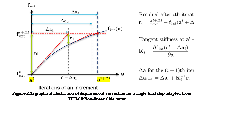
Table 1: Computational flow in a non-linear finite element code adapted from De Brost et al.2012

 

3.     NUMERICAL EXAMPLE OF A STEEL BEAM SUBJECTED TO LOW-SPEED IMPACT LOAD

 

A numerical simulation of a 30m long steel beam (UB  with a thickness of) subject to high-speed impact based on the non-linear theoretical framework discussed above was carried out to investigate the deformation and rotation capacity of the steel beam under the impact.

For this finite element (F.E) simulation, the full Newton-Raphson method was used. The material parameters are as follows:

 

For steel:

·      Young’s Modulus of elasticity;  

·        Poisson ratio                                     0.3

·      Yield stress               

·        Density                                              8E-9

For rigid impactor:

·        Young’s Modulus of elasticity;

·        Poisson ratio                                      0.2

·      Density       

 

The displacement history time graph represents the true characteristic nature of dynamic behaviour for a high frequency (33) loading where the unloading cycle appears to be less than I/10000^th of a second. This unloading time suggests that the impact load is quite severe as the release of instantaneous energy can be assumed from the sharp rise in deformation of the beam of almost. This deformation encompasses the initial vertical downward displacement, the rebound of the beam in the opposite direction (see fig. 4.2) as well as subsequent twisting of the beam.

Figure 3: Time history graph

 

 

Figure 4:  Deformation after initial drop

Figure 4.1: Deformation after initial drop

Figure 4.2: Rebound displacement

 

4.     NUMERICAL SIMULATION

 

After the initial displacement as shown in fig.4 and fig. 4.1 above and the rebound displacement of the beam as shown in fig. 4.2, the beam continued to vibrate. The amplitude of the vibration reduced to zero in less than a second as can be seen from fig. 3. This suggests that the structure is overdamped as the displacement had decayed rather exponentially. The vibration of the structure after impact is as shown in figs. 5 to 7. From the frequency (33) and speed of loading as shown in fig. 3, it shows that the beam is able to respond in a rather ductile manner to the impact loading of a  rigid impactor dropped from a height of  However, from the deformed shape of the beam element after the impact load, it is considered to have failed as its structural integrity is lost due to excessive twisting of the beam.

Similarly, from the initial drop as shown in fig. 2.1, the beam rotated by  and for the rebound displacement the rotation was  which is clearly over the maximum limit to avoid any secondary hazard. Furthermore, the rotation at first mode was  which is clearly above the maximum rotation value of  for steel structures to prevent collapse. Implying that the beam has failed.

 

Figure 4.3: Mode shape 1 rotation

 

 

 

Figure 6:  Mode shape 2

 

Figure 7:  Mode shape 3

 

4.1. ANALYTICAL COMPARISM

 

From the above numerical simulations, the rigid impactor was only in contact with the beam for a short period of time followed by a rebound of the beam due to action of elastic interface restoring force (Aliyu 2019). This according to Stronge (2018) can be classified as an elastic impact. Also form the Newtons experimental law of impact, the coefficient of restitution for an elastic impact is assumed to be 1 (Stronge, 2018). Hence, the kinetic energy for the above elastic impact with a coefficient of restitution 1, according to Mughal and Smith cited in Aliyu (2019), is evaluated using the following expression

 

 

While the maximum vertical downward displacement  as well as the available strain energy  was evaluated using the following expressions

 

The maximum allowable vertical downward displacement was equally evaluated using the following expression

 

 

From the above expressions, the maximum vertical downward deflection as well as the allowable maximum vertical downward deflection were both found to be. This closely matched the initial vertical downward displacement from the Abaqus simulations which was found to be  (see fig. 4)

 

5.     CONCLUSION

     

In a pursuit to analyse non-linear dynamic problems the framework for the displacement based finite element method was introduced where material and geometric non-linearity had been considered. Similarly, the incremental analysis procedure for non-linear problems have been discussed. The accuracy of the results of deformation obtained from this non-linear finite element analysis was compared to those obtained from the analytical technique using the energy momentum balance technique as presented by Mughal and Smith cited in Aliyu (2019) which gave a maximum vertical downward deflection of after initial impact. This was found to agree with the Abaqus vertical downward deflection of  after initial impact. Although, the deflection appeared to be within the acceptable limits, the beam was considered to have failed as the rotation limits for safe design had been exceeded. It has turned out that this displacement-based method of non-linear finite element analysis as well as the energy momentum balance technique presented in (Aliyu, 2019) are viable for use practically as it is able to predict with  accuracy the behaviour of structures subject to impact load (which is a non-linear dynamic problems) at a very reasonable cost.

 

SOURCES OF FUNDING

 

This research received no specific grant from any funding agency in the public, commercial, or not-for-profit sectors.

 

CONFLICT OF INTEREST

 

The author have declared that no competing interests exist.

 

ACKNOWLEDGMENT

 

None.

 

REFERENCES

 

    [1]       Aliyu, OH.  Design Recommendations for Steel Beams to Prevent Brittle Fracture. Nigerian              Journal of Technologycal Development, 16 (2), 2019, 78-84.

    [2]       Aliyu, OH. A Review on Mechnics of Impacts on Steel Plates. Journal of Engieering   Research, Special Edition, 24(1), 2019, 11-28

    [3]       Belytschko, T., Liu, WK., Moran, B., Elkhoday, K I.  Nonlinear Finite Element for Continuua and Structures. Second Edition ed. West Sussex United          Kingdom: John Wiely and Sons. 2014.

    [4]       Stein, E. Progress in Computational Analysis of Inelastic Structures. New York. Springer 1993.

    [5]       Laursen, AT. Computational Contact and Impact Mechanics 2nd Edition. Springer U.S.A, 2003.

    [6]       De Borst, R., Crisfileld, MAR., Remmers, JJC., & Verhrosel, CV. Non-linear Finite Element Analysis of Solid and Structures 2nd Edition.  Johon Wiley and Sons Ltd. United Kingdom, 2012.

    [7]       Mughal, MA, Smith, SJ. Design Guide for Structures Subject to Impulse and Impactive Loads. PPG Report No. SXB-IC-096565; NDA Report No. PWR/92/161 Bechtel Guide No. C-2.45 1994.

    [8]       Stronge, WJ. Impact Mechanics First ed. Cambridge United: Cambridge University Press. 2018.

    [9]       Seshu, P.  Finite Element Analysis. PHI Learning Private Limited New Delhi, 2012.

  [10]      Wang, T., Hsu, TTC. Nonlinear finite element analysis of concrete structures using new consitiutive models. Computer and Structures 79, 2001, 2781-2791.

  [11]     Ayoub, A. & Filippou, FC. Nonlinear Finite Element Analysis of R.C. Shear Panels and Walls. Journal of Structural Engineering, 124, 1998, 298-308.

  [12]     Kim, N. Introduction to Nonlinear Finite Element Analysis. Springer New York, 2018.

  [13]      Hartmann, S. A remark on te application of the Newton-Raphson method in non-linear finite element analysis. Computer Mechanics. 36, 2005, 100-116.

  [14]     Tsavadaris, KD. & Mello, CD. Vierendeel Bending Study of Perforated Steel Beams with Various Novel Web Opening Shapes Through Non-linear Finite Element Analysis. Journal of Structural Engineering, 138 (10), 2012, 1214-1230.

  [15]     Barth, B K.  & Wu, H. Efficient nonlinear finite element modelling of slab on steel stringer bridges. Elsevier, 2006, 1304-1313.