TIME-OPTIMAL PATH PLANNING MODEL USING GENETIC ALGORITHM IN RRR ROBOT

Hasan Demir; Mehmet R. Tolun; Filiz Sari

doi:10.29121/ijetmr.v8.i5.2021.938

TIME-OPTIMAL PATH PLANNING MODEL USING GENETIC ALGORITHM IN RRR ROBOT

Hasan Demir ✉

¹ , Mehmet R. Tolun

² , Filiz Sari

1 Ortaköy Vocational School, Aksaray University, Turrkey

2 Department of Computer Engineering, Konya Food and Agriculture University, Turkey

3 Aksaray University, Department of Electrical and Electronics Engineering, Turkey

How to cite this article (APA): Demir, H, Tolun, MR, & Sari, F (2021). Time-optimal path planning model using genetic algorithm in rrr robot. International Journal of Engineering Technologies and Management Research, 8(5), 9. doi: 10.29121/ijetmr.v8.i5.2021.938

Abstract

The mathematical expression of the kinematic equations of each joint is utilized for the path planning using a quantic polynomial in joint space. In this study, a time optimization model for path planning using genetic algorithms with a variety of crossover fraction and mutation rates is investigated. The optimization process is performed with MATLAB. Optimization using boundary conditions is performed with MATLAB. The result of the simulation, smooth speed graphs, angular position graphs, and the time when joint movements will complete the orbit as soon as possible are obtained. As a result of this study, a path planning model that can be applied to any robot is developed in joint space based on time optimization and can be used to shorten the task time, especially in task-based robots.

Keywords

Path Planning, Genetic Algorithm, Time Optimization

INTRODUCTION

Trajectory planning is an important research topic in robot applications, and many research papers are published on this subject (Duque, Prieto, & Hoyos, 2017), (Markus, Agee, & Jimoh, 2013), (Ragaglia, Zanchettin, & Rocco, 2018). Robot trajectory planning means that the end-effector passing through specific points reaches the target point from the starting point. Each joint angle varies depending on the time in trajectory planning. The primary purpose of trajectory planning is to automatically create a collision-free trajectory for the robot by making a motion plan in an environment with obstacles. Trajectory planning can be done in Cartesian space or in Joint space. Trajectory planning in joint space is more straightforward than in Cartesian space. To make trajectory planning in joint space, the points given in Cartesian space must be found in the joint space using inverse kinematics. Robot trajectory planning research analyzes the velocity and acceleration of each joint. The mechanical properties of the robots determine the limits of the velocity and acceleration of the joints. For this reason, research is done on improving trajectory planning (Haiek, Aboulissane, Bakkali, & Bahaoui, 2019), (Jin, Kang, Zhang, & Yang, 2016), (Tan & Hu, 2002), (Zhang, Meng, Feng, & Shen, 2018).

The purpose of the methods generally used in trajectory planning is to avoid complex geometric processes (Abu-Dakka, Rubio, Valero, & Mata, 2013), (Machmudah, Parman, Zainuddin, & Chacko, 2013), (Mineo, Pierce, Nicholson, & Cooper, 2016), to reduce the processing time, to make the shortest trajectory planning (Cao, Jiang, & Yue, 2017), (Chen, Fang, Sun, & Qian, 2015), (Gasparetto & Zanotto, 2010), (Gu, Cai, Hu, Zhang, & Chen, 2019), (Kim & Kim, 2011), (Ko, Ryuh, Kim, Suprem, & Mahalik, 2015), (Xu, Xie, Zhuang, & Wang, 2010), and to optimize using different algorithms (Garrido, Yu, & Li, 2016), (Lara-Molina, Koroishi, & Dumur, 2015), (Švejda & Čechura, 0411). The most researched subject among these topics is to improve trajectory planning parameters using optimization techniques. The studies conducted in trajectory planning are mostly done in joint space because it is intuitive and straightforward. In addition, trajectory planning is carried out using polynomial interpolation algorithms in the joint space because these algorithms are not problematic for computing (Cao et al., 2017). The movements of the robot must be smooth and continuous without vibration. For this reason, the B-spline curve is generally used in interpolation methods, and optimum processing time and angular displacement, velocity, and acceleration graphs for each joint are found in trajectory planning studies (Gasparetto et al., 2010).

In this study, a trajectory planning model is created for the RRR robot arm based on time optimization. Since the first three joints affect Cartesian space's position, the robot arm in the RRR structure was preferred. Trajectory planning is done with quintic interpolation in the joint space, and time optimization is performed for each joint using a genetic algorithm. Attention has been paid to make the movements of the joints smooth and continuous.

MATERIALS AND METHODS

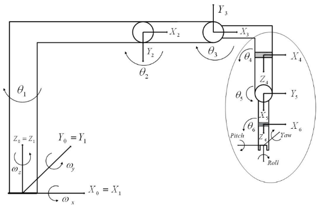
Today, robots with six degrees of freedom (DOF) illustrated in Figure 1 are used in the industry because of their speed and flexibility. Mathematical models of robot arms contain highly nonlinear equations. The most common method for controlling robots is by looking at the look-up tables (Deshpande & George, 2014). The robot arms consist of interconnected links. Connections consist of revolute or prismatic joints. The relationship between the joints is defined by 4x4 transformation matrices. By multiplying these matrices, the matrix containing the final orientation and position obtained, and this process is called forward kinematics (Craig, 2004). Forward kinematic equations are simple and do not have complex equations (Schilling, 1990). It is passed from Cartesian space to joint space with the forward kinematic, while the inverse kinematic provides the transition from the joint space to the Cartesian space. The solution for going from point A to point B in Cartesian space is found with inverse kinematics. There are two methods for solving inverse kinematics which is the numerical solution and the closed-form. The closed-form is more preferred because it runs faster (Küçük, Kocaeli, & Bingül, 2004). There is only one general method to solve robot kinematics which is Denativ-Hartenberg (D-H) (Huang, Wang, Liu, & Cui, 2012), (Li, Cao, Guo, & Huang, 2015), (Redondo & LeSar, 2004).

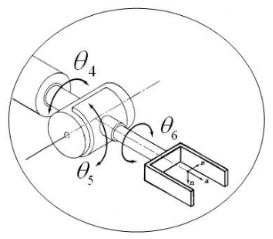
The last three joints that make up the wrist structure are identical, but the first three joints that affect the position are different in industrial robots. The first three joints' joint properties are essential to classify the robots according to DOF (Bingül & Küçük, 2009). The first three joints determine the robot's position in Cartesian space, while the last three joints (Euler's wrist) define the robot's orientation, and the Euler's wrist is illustrated in Figure 2 .

https://www.granthaalayahpublication.org/journals-html-galley/html-images/c127ddcb-4d62-494f-8751-43eaf6872e10image1.png — **Figure 1: 6-DOF industrial robot arm (Hasan, 2010)**

The D-H table of the Euler's wrist is given in Table 1 , and the D-H parameters are the same for industrial robots.

https://www.granthaalayahpublication.org/journals-html-galley/html-images/c127ddcb-4d62-494f-8751-43eaf6872e10image2.png — **Figure 2: Euler wrist (Hasan, 2010)**

Table 1: The D-H table of the Euler wrist (Bingül et al., 2009)

i	α_i-1	a_i-1	d_i	θ_i
1	0	0	0	θ₄
2	90	0	0	θ₅
3	-90	0	0	θ₆

In this study, three rotary joints are used in the robot configuration. This configuration is the basis of most industrial robots because they have a vast working space, and they are very flexible and fast. But their kinematic equations have very complicated. The robot configuration and the coordinate frames which are shown in Figure 3 has the three-rotary joint.

https://typeset-prod-media-server.s3.amazonaws.com/article_uploads/c40d7f75-9d35-45bd-b2c9-3c633d2552d7/image/2ec9de3f-8dd3-4246-b0b0-0cf36e4cacca-uimage.png — **Figure 3: a) Therobot configuration, b) The coordinate frames**

D-H method uses four main variables, which are the bond length between two axes ( $a_{i - 1}$ ), the bond angle between axes (i-1) and i ( $α_{i - 1}$ ), the joint misalignment between overlapping bonds ( $d_{i}$ ), and the joint angle between two bonds ( $θ_{i}$ ). The D-H variables for our design are shown in Table 2 .

Table 2: D-H variables for the robot

Number of axes	D-H variables				Joint variables
i	$α_{i - 1}$	$a_{i - 1}$	$d_{i}$	$θ_{i}$	$d_{i} or θ_{i}$
1	0	0	D₁	$θ_{1}$	$θ_{1}$
2	-90	0	L₁	$θ_{2}$	$θ_{2}$
3	0	L₂	0	$θ_{3}$	$θ_{3}$
4	0	L₃	0	0	0

The transformation matrix of a joint is obtained by using Equation 1 .

{{}^{i - 1}T}_{i} = (\begin{matrix} c θ_{i} & - s θ_{i} & 0 & a_{i - 1} \\ s θ_{i} c α_{i - 1} & c θ_{i} c α_{i - 1} & - s α_{i - 1} & - s α_{i - 1} d_{i} \\ s θ_{i} s α_{i - 1} & c θ_{i} s α_{i - 1} & c α_{i - 1} & c α_{i - 1} d_{i} \\ 0 & 0 & 0 & 1 \end{matrix}]

The transformation matrices for each joint are given by:

0 T_{1} = (\begin{matrix} c_{1} & - s_{1} & 0 & 0 \\ s_{1} & c_{1} & 0 & 0 \\ 0 & 0 & 1 & d_{1} \\ 0 & 0 & 0 & 1 \end{matrix}]

1 T_{2} = (\begin{matrix} c_{2} & - s_{2} & 0 & 0 \\ 0 & 0 & 1 & l_{1} \\ - s_{2} & - c_{2} & 0 & 0 \\ 0 & 0 & 0 & 1 \end{matrix}]

2 T_{3} = (\begin{matrix} c_{3} & - s_{3} & 0 & l_{2} \\ s_{3} & c_{3} & 0 & 0 \\ 0 & 0 & 1 & 0 \\ 0 & 0 & 0 & 1 \end{matrix}]

3 T_{4} = (\begin{matrix} 1 & 0 & 0 & l_{3} \\ 0 & 1 & 0 & 0 \\ 0 & 0 & 1 & 0 \\ 0 & 0 & 0 & 1 \end{matrix}]

The forward kinematic matrix is obtained by multiplying the transformation matrices.

{}_{4}^{0}T = {}_{1}^{0}T {}_{2}^{1}T {}_{3}^{2}T {}_{4}^{3}T {}_{4}^{0}T = (\begin{matrix} r_{11} & r_{12} & r_{13} & p_{x} \\ r_{21} & r_{22} & r_{23} & p_{y} \\ r_{31} & r_{32} & r_{33} & p_{z} \\ 0 & 0 & 0 & 1 \end{matrix}]

The analytical solution approach is used for inverse kinematic solution. In this solution, r_ij is the rotation, and px, py, pz is the position specifying elements.

The forward kinematic matrix is written in Equation 6 as symbolically. Both sides of the equation are multiplied by ${({}_{1}^{0}T]}^{- 1}$ .

{}_{4}^{0}T {({}_{1}^{0}T]}^{- 1} = {({}_{1}^{0}T]}^{- 1} {}_{1}^{0}T {}_{2}^{1}T {}_{3}^{2}T {}_{4}^{3}T {}_{4}^{0}T {({}_{1}^{0}T]}^{- 1} = {}_{2}^{1}T {}_{3}^{2}T {}_{4}^{3}T

When Equation 7 is solved, the joint variables are found.

θ_{1} = A t a n 2 (- p_{x}, p_{y}) + A t a n 2 (\mp \sqrt{p_{x}^{2} + p_{y}^{2} - l_{1}^{2}}, l_{1})

\begin{array}{l} θ_{3} = A t a n 2 (\mp \sqrt{1 - {(\frac{p_{x}^{2} + p_{y}^{2} + (p_{z} - d_{1})^{2} - l_{3}^{2} - l_{2}^{2}}{2 l_{3} l_{2}})}^{2}} \\ , \frac{p_{x}^{2} + p_{y}^{2} + (p_{z} - d_{1})^{2} - l_{3}^{2} - l_{2}^{2}}{2 l_{3} l_{2}}) \end{array}

\begin{array}{l} \begin{array}{l} θ_{2} = A t a n 2 (- l_{3} c o s (θ_{3}) - l_{2}, - l_{3} s i n (θ_{3})) \mp \\ . . . A t a n 2 (\sqrt{l_{3}^{2} + l_{2}^{2} + 2 l_{3} l_{2} c o s (θ_{3}) - (p_{z} - d_{1})^{2}}, p_{z} - d_{1}) \end{array} \end{array}

TRAJECTORY PLANNING

The trajectory planning is performed with three or higher-order polynomials in joint space. The inverse kinematic solution gives the initial and target positions of the end effector. A quantic (5-degree) polynomial is needed to obtain smoothing the path curve, shown in Equation 11 (Tan et al., 2002).

θ (t) = s_{0} + s_{1} t + s_{2} t^{2} + s_{3} t^{3} + s_{4} t^{4} + s_{5} t^{5}

At the start and endpoint, the velocity, acceleration, and displacement limits are given by:

θ (0) = θ_{0} θ (f) = θ_{f}

θ^{'} (0) = θ_{0}^{'} θ^{'} (f) = θ_{f}^{'}

θ^{″} (0) = θ_{0}^{″} θ^{″} (f) = θ_{f}^{″}

The velocity polynomial is obtained from the derivation of Equation 11. It is possible to find the acceleration equation by taking the derivation of the velocity polynomial. The coefficients of the angular position equation can be determined by:

s_{0} = θ_{0}

s_{1} = θ_{0}^{'}

s_{5} = \frac{12 (θ_{f} - θ_{0}) - 6 (θ_{f}^{'} + θ_{0}^{'}) t_{f} - (θ_{0}^{″} - θ_{f}^{″}) t_{f}^{2}}{2 t_{f}^{5}}

s_{2} = \frac{θ_{0}^{″}}{2}

s_{3} = \frac{20 (θ_{f} - θ_{0}) - (8 θ_{f}^{'} + 12 θ_{0}^{'}) t_{f} - (θ_{f}^{″} - 3 θ_{0}^{″}) t_{f}^{2}}{2 t_{f}^{3}}

s_{4} = \frac{30 (θ_{f} - θ_{0}) - (14 θ_{f}^{'} + 16 θ_{0}^{'}) t_{f} + (3 θ_{0}^{″} - 2 θ_{f}^{″}) t_{f}^{2}}{2 t_{f}^{4}}

SIMULATION USING GENETIC ALGORITHMS

The technical characteristics of the electric motors used in the joints directly affect the path planning. Genetic algorithms are used for optimal path planning using the limits of electric motors.

Each robot arm reaches its target point by passing through n points. Therefore, the motion of each joint should be examined separately. If one of the joints completes its motion in ti time, the total motion time is expressed in Equation 16.

T = \sum t_{i}

The evolutionary Genetic Algorithm (G.A.) has been used to optimize the motion time. The objective function used in experimental studies to complete a certain movement as soon as possible is given in Equation 17.

Objective Function: ​ T = \sum t_{i}

hows the constraint conditions of the objective function. The constraint conditions determine the technical characteristics of the servo motors used in the joints.

Table 3: The constraint conditions

Joint	$Velocity θ^{'} (t)$	$Acceleration θ^{″} (t)$
1	$300 \leq θ^{″} (t) \leq 600$	$50 \leq θ^{″} (t) \leq 200$
2	$300 \leq θ^{″} (t) \leq 600$	$50 \leq θ^{″} (t) \leq 200$
3	$400 \leq θ^{″} (t) \leq 750$	$40 \leq θ^{″} (t) \leq 300$

In the optimization, selection mechanisms have determined scholastic uniformly. The population size is chosen as 200. Optimization was performed at different mutation rates and crossover fractions to achieve the best objective function. The crossover fraction is selected as 0.2, 0.5, and 0.8. Mutation rates are chosen as 0.01 and 0.02.P₀ (X₀ = 155.28, Y₀ = 0, Z₀ = 164.14) to P₁ (X₁ = 135.65, Y₁ = 23.92, Z₁ = 99.12)[HD1] In the simulation, the robot arm was moved from

Table 4: The result of optimizations with different mutation rates and different crossover fractions.

Crossover Fraction	Mutation Rate of the First Joint		Mutation Rate of the Second Joint		Mutation Rate of the Third Joint
Crossover Fraction	0.01	0.02	0.01	0.02	0.01	0.02
0.2	4.24358 sec	4.24654 sec	5.21699 sec	5.20255 sec	4.90852 sec	4.92415 sec
0.5	4.2516 sec	4.28907 sec	5.27448 sec	5.19656 sec	4.94927 sec	4.94372 sec
0.8	4.24369 sec	4.28733 sec	5.20639 sec	5.19776 sec	4.91203 sec	4.94527 sec

Considering that the joints move sequentially, the robot completes the arm movement in 14.346 seconds. This period is sufficient for the robot to perform its movement smoothly as it is calculated as the shortest time in tests.

CONCLUSIONS

In this study, the path planning for a specific movement in the joint space of a robot with RRR joint structure is considered. Since the first three joints in 6 joint industrial robots determine the position in Cartesian space, the robot structure in this study consists of three joints. The quintic path polynomial is created for the specified motion. Time optimization is realized with G.A. The constraint conditions used in optimization were velocity and acceleration, and the movements are provided to be smooth. The best objective function is found by diversifying the optimization parameters. In reference (Zhang et al., 2018), the path planning method in joint space is defined using genetic algorithms for PUMA 560 robot model. Optimization studies were made for a robot model. In this study, a time optimization model is developed using G.A. for industrial robot arms. The shortest working time of each joint is found for the specified movement. The time optimization model developed can reduce task time for robot structures designed to work fast, such as delta robots. The algorithm developed can be used to increase product output by shortening the task times of task-based robots.

[1] Abu-Dakka, F. J., Rubio, F., Valero, F. & Mata, V. (2013). Evolutionary indirect approach to solving trajectory planning problem for industrial robots operating in workspaces with obstacles. European Journal of Mechanics - A/Solids 42, 210–218. Retrieved from https://dx.doi.org/10.1016/j.euromechsol.2013.05.007 10.1016/j.euromechsol.2013.05.007

[2] Bingül, Z. & Küçük, S. (2009). Kinematic Of Robot. İstanbul: Birsen Yayınevi

[3] Cao, K.-C., Jiang, B. & Yue, D. (2017). Cooperative path following control of multiple nonholonomic mobile robots. ISA Transactions 71, 161–169. Retrieved from https://dx.doi.org/10.1016/j.isatra.2017.06.028 10.1016/j.isatra.2017.06.028

[4] Chen, H., Fang, Y., Sun, N. & Qian, Y. (2015). Pseudospectral Method Based Time Optimal Trajectory Planning For Double Pendulum Cranes. Chinese Control Conference, CCC, 2015-Septe 4302–4307.

[5] Craig, J. J. (2004). 2.Introduction To Robotics Mechanics And Control. Prentice Hall 1 Retrieved from Https://Doi.Org/10.1109/MEX.1986.4306961

[6] Duque, D. A., Prieto, F. A. & Hoyos, J. G. (2017). Trajectory Generation For Robotic Assembly Operations Using Learning By Demonstration. Robotics And Computer-Integrated Manufacturing 57, 292–302.

[7] Garrido, J., Yu, W. & Li, X. (2016). Robot trajectory generation using modified hidden Markov model and Lloyd's algorithm in joint space. Engineering Applications of Artificial Intelligence 53, 32–40. Retrieved from https://dx.doi.org/10.1016/j.engappai.2016.03.006 10.1016/j.engappai.2016.03.006

[8] Gasparetto, A. & Zanotto, V. (2010). Optimal trajectory planning for industrial robots. Advances in Engineering Software 41(4), 548–556. Retrieved from https://dx.doi.org/10.1016/j.advengsoft.2009.11.001 10.1016/j.advengsoft.2009.11.001

[9] Gasparetto, A. & Zanotto, V. (2008). A technique for time-jerk optimal planning of robot trajectories. Robotics and Computer-Integrated Manufacturing 24(3), 415–426. Retrieved from https://dx.doi.org/10.1016/j.rcim.2007.04.001 10.1016/j.rcim.2007.04.001

[10] Gu, W., Cai, S., Hu, Y., Zhang, H. & Chen, H. (2019). Trajectory planning and tracking control of a ground mobile robot:A reconstruction approach towards space vehicle. ISA Transactions 87, 116–128. Retrieved from https://dx.doi.org/10.1016/j.isatra.2018.11.019 10.1016/j.isatra.2018.11.019

[11] Haiek, D. E., Aboulissane, B., Bakkali, L. E. & Bahaoui, J. E. (2019). Optimal Trajectory Planning for Spherical Robot Using Evolutionary Algorithms. Procedia Manufacturing 32, 960–968. Retrieved from https://dx.doi.org/10.1016/j.promfg.2019.02.309 10.1016/j.promfg.2019.02.309

[12] Hasan, A. T. (2010). Performance Prediction Network For Serial Manipulators Inverse Kinematics Solution Passing Through Singular Configurations. 7, 10–23

[13] Huang, J., Wang, X., Liu, D. & Cui, Y. (2012). A New Method For Solving Inverse Kinematics Of An Industrial Robot. International Conference On Computer Science And Electronics Engineering 3, 53–56.

[14] Jin, X., Kang, J., Zhang, J. & Yang, X. (2016). Trajectory Planning Of A Six-DOF Robot Based On A Hybrid Optimization Algorithm. Retrieved from Https://Doi.Org/10.1109/ISCID.2016.148

[15] Kim, K. B. & Kim, B. K. (2011). Minimum-Time Trajectory For Three-Wheeled Omnidirectional Mobile Robots Following A Bounded-Curvature Path With A Referenced Heading Profile. IEEE Transactions On Robotics 27(4), 800–808.

[16] Ko, M. H., Ryuh, B.-S., Kim, K. C., Suprem, A. & Mahalik, N. P. (2015). Autonomous Greenhouse Mobile Robot Driving Strategies From System Integration Perspective: Review and Application. IEEE/ASME Transactions on Mechatronics 20(4), 1705–1716. Retrieved from https://dx.doi.org/10.1109/tmech.2014.2350433 10.1109/tmech.2014.2350433

[17] Küçük, S., Kocaeli, U. & Bingül, Z. (2004). The Inverse Kinematics Solutions Of Industrial Robot Manipulators. Mechatronics, 2004. ICM ’04. Proceedings Of The IEEE International Conference On. 274–279 Retrieved from Https://Doi.Org/10.1109/ICMECH.2004.1364451

[18] Lara-Molina, F. A., Koroishi, E. H. & Dumur, D. (2015). Combined Structure-Control Optimal Design Of The Stewart-Gough Robot. 12th Latin American Robotics Symposium And 2015 3rd Brazilian Symposium On Robotics (LARS-SBR) 19–24.

[19] Li, W. B., Cao, G. Z., Guo, X. Q. & Huang, S. D. (2015). Development Of A 4-DOF SCARA Robot With 3R1P For Pick-And-Place Tasks. 6th International Conference On Power Electronics Systems And Applications: Electric Transportation - Automotive, Vessel And Aircraft, PESA 2015 .

[20] Li, Z., Li, G., Sun, Y., Jiang, G. & Jianyi, K. (2017). Development Of Articulated Robot Trajectory Planning. 8, 52–60 Retrieved from Https://Doi.Org/10.1504/IJCSM.2017.083152

[21] Machmudah, A., Parman, S., Zainuddin, A. & Chacko, S. (2013). Polynomial joint angle arm robot motion planning in complex geometrical obstacles. Applied Soft Computing 13(2), 1099–1109. Retrieved from https://dx.doi.org/10.1016/j.asoc.2012.09.025 10.1016/j.asoc.2012.09.025

[22] Markus, E. D., Agee, J. T. & Jimoh, A. A. (2013). Trajectory Control Of A Two-Link Robot Manipulator In The Presence Of Gravity And Friction. Retrieved from Https://Doi.Org/10.1109/AFRCON.2013.6757809

[23] Mineo, C., Pierce, S. G., Nicholson, P. I. & Cooper, I. (2016). Robotic path planning for non-destructive testing – A custom MATLAB toolbox approach. Robotics and Computer-Integrated Manufacturing 37, 1–12. Retrieved from https://dx.doi.org/10.1016/j.rcim.2015.05.003 10.1016/j.rcim.2015.05.003

[24] Ragaglia, M., Zanchettin, A. M. & Rocco, P. (2018). Trajectory generation algorithm for safe human-robot collaboration based on multiple depth sensor measurements. Mechatronics 55, 267–281. Retrieved from https://dx.doi.org/10.1016/j.mechatronics.2017.12.009 10.1016/j.mechatronics.2017.12.009

[25] Redondo, A. & LeSar, R. (2004). MODELING AND SIMULATION OF BIOMATERIALS. Annual Review of Materials Research 34(1), 279–314. Retrieved from https://dx.doi.org/10.1146/annurev.matsci.34.070503.123908 10.1146/annurev.matsci.34.070503.123908

[26] Schilling, R. J. (1990). Fundamentals Of Robotics. USA: Prentice Hall

[27] Švejda, M. & Čechura, T. (0411). Interpolation Method For Robot Trajectory Planning. Proceedings Of The 2015 20th International Conference On Process Control, PC 2015 .

[28] Tan, G. Z. & Hu, S. Y. (2002). Real-Time Accurate Hand Path Tracking And Joint Trajectory Planning For Industrial Robots (II) Journal Of Central South University Of Technology (English Edition) 9(4), 273–278.

[29] Vivek Deshpande, &. P. M. & George, (2014). Kinematic Modelling And Analysis Of 5 DOF Robotic Arm. International Journal Of Robotics Research And Development (IJRRD) 4(2), 1–8.

[30] Xu, H., Xie, X., Zhuang, J. & Wang, S. (2010). Global Time-Energy Optimal Planning Of Industrial Robot Trajectories. Journal Of Mechanical Engineering 46(9), 19–25.

[31] Zhang, J., Meng, Q., Feng, X. & Shen, H. (2018). A 6-DOF Robot-Time Optimal Trajectory Planning Based On An Improved Genetic Algorithm. Robotics And Biomimetics 5(1), 3–9.