INTRODUCTION

Many statistical techniques are available for handling various problems. Some of these techniques come as models such as linear, exponential and quadratic models. These models have become integral components concerned with describing the relationship between a response variable and one or more explanatory variables (Hosmer & Lemeshow, 2000). If there is a reason to believe that a linear relationship exists between a variable of interest (response variable) and other variables (predicator variables) in a study, the ordinary linear model is one technique that is often used for predicting outcomes (Alan, 2002). This technique is mostly adopted due to its flexibility for analyzing the relationship between multiple independent variables and a single dependent variable. Much of its flexible is due to the way in which all sorts of independent variables can be accommodated (Joaquim & Sá, 2007).

It is meaningful to address how the analyst can deal with data representing multiple independent variables and a categorical dependent variable, how independent variables can be used to contribute to the discovery of differences in the categories. The assignment of observations or objects into predefined homogenous groups is a problem of major practical and research interest. For example, we may use quantitative information in predicting who will or will not graduate from a college. This would be an example of simple binary classification problems, where the categorical dependent variable can only assume two distinct values. In other cases, there are multiple categories or classes for the categorical dependent variable. For example, when we are ill, we want a doctor to diagnose our disease from the symptoms of the illness, the outcome maybe more than two.

All the above are classification problems where we attempt to predict values of a categorical dependent variable from one or more continuous and/or categorical predictor variables. In statistics, it is the process of allocating an observation p in one of several predefined groups or categories and an ideal classification method which distinguishes different classes from each other. The basic objective is to build a discriminant function that takes the information to summarize the p variables on an indicator that yields the optimal discrimination between the classes − the goal of classification in this case − also known as supervised pattern recognition (Wehrens, 2010). In order to derive the decision rule that yields the optimal discrimination between the classes, one assumes that a training set of pre-classified cases −the data sample− is available, and can be used to determine the model applicable to new cases. The decision rule can be derived in a model-based approach, whenever a joint distribution of the random variables can be assumed, or in a model-free approach (Joaquim et al., 2007).

There are numerous algorithms for predicting continuous or categorical variables from a set of continuous predictors and/or categorical factor effects (Lewicki & T, 2006). For example, in GLM (General Linear Models) and GRM (General Regression Models), we can specify a linear combination design of continuous predictors and categorical factor effects to predict a continuous dependent variable. In GDA (General Discriminant Function Analysis), we can specify such designs for predicting categorical variables to solve classification problems.

A neural-network is a classification algorithm in the field of artificial intelligence. It is a very powerful tool with the capability of pattern recognition. Artificial Neural Networks (ANNs) were designed to model the functioning of human brain. Linear classifiers separate objects by the value of a linear combination of their features. The feature of an object is represented by a vector. There is another vector to be trained with known observations. This is called weight vector. There are several algorithms in this category such as Support Vector Machines (SVM, Multi-layer Perceptron (MLP) and the radial Basis Function (RBF).

The objective of this work is to evaluate the implementation and performance of classification techniques (a multi-layer perceptron) comparatively with a logistic regression model, in order to predict the presence of diabetes in a collected data from Federal Medical Center, Yola, Adamawa State, Nigeria. This paper describes how these techniques have been applied to the data and presents a comparison analysis. The results are reported and discussed according to this technique.

MATERIALS AND METHODS

Between 1^st August, 2016 to 31^st October, 2017, a total of five hundred and fifty-three (553) women were tested for diabetes at FMC, Yola. Three hundred and six were diabetic while two hundred and forty-seven were non diabetic. The data collected was from records of patients at FMC, YOLA.

Observation with missing data were dropped from the analysis. The final dataset consists of 553 subjects, described by several clinical characteristics.

The classification task consists of predicting whether a patient would test positive for diabetes. The class labels of the data are 1 for diabetes and 0 otherwise. There are 8 predictor variables for 553 patients.

The data set have the following numeric attributes and they are:

• “glucose”: Plasma glucose concentration 2 hours in an oral glucose tolerance test.

• “pressure”: Diastolic blood pressure (mm Hg)

• “insulin”: 2-Hour serum insulin (mu U/ml).

• “mass”: Body mass index (weight in kg/(height in meters)

• “age”: Age in years.

• Class variable (0 or 1). The Class variable (6) is treated as 0 (false), 1 (true – tested positive for diabetes).

APPLICATION OF CLASSIFICATION TECHNIQUES.

Two classification techniques were used to fit a prediction model to the data; logistic regression and a multi-layer perceptron. This fitting process is hereby described for each method.

Logistic Regression model

Consider a random variable W that can take either of the two possible values. Given a dataset with a total sample size of M, where each observation is independent, W can be assumed as a On the prevalence of diabetes mellitus in the North Western Part of Nigeria 4 column vector of M binomial random variables Wi. By convention, a value of 1 is used to designate” success" and a value of 0 used to signify “failure." To simplify computational details of estimation, it is convenient to aggregate the data such that each row represents one distinct combination of values of the independent variables. These rows are often referred to as “populations." Let N represent the total number of populations and let n be a column vector with elements ni representing the number of observations in population i for i = 1 to N and M, the total sample size. Now, let Y be a column vector of length N where each element Yi is a random variable representing the number of successes of W for the population. Let column vector y contain elements yi representing the observed counts of the number of successes for each population. Let be a column vector also of length N with elements ${\pi }_i=p(w_i= \frac{1}{i})$ , i.e., the probability of success for any given observation in the ith population. The linear components of the model enclose design matrix and the vector of parameters to be projected. The design matrix of independent variables, X, is composed of N rows and K + 1 columns, where K is the number of explanatory variables speci_ed in the model, for each row of the design matrix, the first element $x_{io}=1$ . This is the intercept or “alpha”. The parameter vector, is a column vector of length K + 1. There is one parameter equivalent to each

of the K columns of independent variable settings in X, plus one ${\beta }_0$ , for the intercept. The logistic regression model equates the log it transforms, the log-odds of probability of a success, to the linear component:

Where $\left(\frac{{\pi }_i}{1-{\pi }_i}\right)$ is known as the odds of an event. Suppose y takes the values 1 for an event and 0 for a non-event, hence y has a Bernoulli distribution with probability parameter (and expected value) p.

Parameter estimation

The goal of logistic regression is to estimate the K + 1 unknown parameters $\beta$ in (1). This is done with maximum likelihood estimation, which entails finding the set of parameters for which the probability of the observed data is greatest. The maximum likelihood equation is derived from the probability distribution of the dependent variable. Since each yi represents a binomial count in the ith population, the joint probability density function of Y is:

For each population, there are different ways to arrange yi successes from ni trails. Since the probability of success for any of ni trails is ${\pi }_i$ , the probability of yi successes is ${\pi }_i^{y_i}$ . Likewise, the probability of $n_i-y_i$ is ${(1-{\pi }_i)}^{n_i-y_i}$ . The joint probability densities function in (2) expresses the values of y as a function of known fixed values for $\beta$ . Thus,

The maximum likelihood estimates are the values for $\beta$ that maximize the likelihood function in (3). Thus, finding the maximum likelihood estimates requires computing the first and second derivatives of the likelihood function. Attempting to take the derivative of (3) with respect to $\beta$ , and after rearranging terms, the equation to be maximized can be written as:

Recall that:

After taking exponent on both sides, equation (5) becomes:

After solving for ${\pi }_i$ it becomes

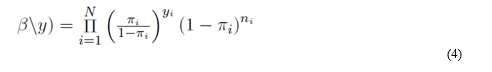
Substituting (6) for the first term and (7) for the second term, equation (4) becomes:

Simplifying the product on the right-hand side in (8), it can be now be written as:

This is the kernel of the likelihood function to maximize. However, it is still cumbersome to differentiate and can be simplified a great deal further by taking its log. Since the logarithm is a monotonic function, and a maximum of the likelihood function will also be a maximum of the log-likelihood function and vice versa. Thus, taking the natural log (9) yields the log-likelihood function:

To find the critical points of the log-likelihood function, set the _rst derivative with respect to each equal to zero. In differentiating (10), we note:

Thus (10) becomes:

The maximum likelihood estimate $\beta$ can be found by setting, each of the K+1 in (12) to zero and solving for each ${\beta }_k$ : By differentiating for the second time; thus:

Solving (13) further by rules of differentiation:

And (14) can now be written as:

Having verified that, the matrix of second partial derivatives is negative definite and the solution is a global maximum, rather than a local maximum. Then we conclude that this vector contains the parameter estimates for which the observed data would have the highest probability of occurrence. This solution has to be numerically estimated using an iterative process, perhaps using Newton's method for solving nonlinear equations. Setting (12) equal to zero results in the system of a K+1 unknown variable _k. Recall that, the Taylor polynomial of degree n forf the point x = x0 is defined as the first n terms of Taylor series for f

Provided that the first n derivatives of f at $x_0$ all exist $x_0{f(x}_0)$ with f(x) = 0

Solving for (x) we have

The value of x is the next approximation for the root. We let x1 = x and continue in the same manner to generate x2, x3 … , until the approximations converge. We write (12) as $l^{\text{'}}\left(\beta \right)$ . Let ${\beta }^0$ represent the vector of initial approximation for each ${\beta }_k$ , and then the first step of Newton-Raphson can be expressed as:

Let $\mu$ be a column vector of length N with the element ${\mu }_i=n_i{\pi }_i: {\mu }_i=E\left(y_i\right)$ the expected value of $y_i$ using matrix multiplication:

Equation (19) is a column vector of length K + 1, whose elements as $\frac{\partial l\left(\beta \right)}{\partial {\beta }_k}$ derived in (11). Now, let W be a square matrix of order N with the element $n_i{\pi }_i (1- {\pi }_i)$ on the diagonal and zeros everywhere else. Again, using matrix multiplication we verify that:

(20) K + 1 by K + 1 square matrix. Now (18) can be written as:

Continue applying (21) until there is essentially no change between the elements of $\beta$ within iterations. At the point; The maximum likelihood estimates are said to be converged, (20) will hold the variance-covariance matrix of the estimate.

Classification accuracy

According to (Muhammad et al., 2018), “The purpose of the classification is to assign a class to discover formerly unseen records as accurately as possible. If there is a group of records (called a training set) and each record contains a set of attributes, then one of the attributes is class (Chao & Wong, 2009), (Podgorelec & Maribor, 2005). The motive is to find a classification model for class attributes, where a test set is used to find out the accuracy of the model. The acknowledged figured set are divided into training and testing sets. The training set used to fabricate the model and testing set is used to authenticate it (Wang & Zhou, 2005), (Karegowda & Jayaram, 2009). classification practice consists of a training set that is analysed by a classification algorithm and the classifier or learner (Tang & Tseng, 2009). Model is represented in the composition of classification rules (Xue & Yanan, 2006)”. Testing data are used in the classification rules to estimate the accuracy. The learner model is represented in the form of classification rules or decision trees.The reference model was built by entry of 5 variables followed by removal of those with no significant partial correlation (R Statistic). The SPSS version 25 for Windows (10.1) was used for these analyses.

The Multi-layer perceptron

We used a common feedforward backpropagation multilayer perceptron (MLP) simulator developed in SPSS software package. The prediction method is based on the nonlinear weighted combination of input units (i.e. predictive variables) to predict one or more output units (i.e. outcome variable). The learning process is iterative and essentially consists in adjusting the weights to decrease the output error. The network was specified with one input layer (representing the five predictive variables), one hidden layer (including five hidden units) and one output layer (with one output unit representing a binary diabetic event). Several sensitivity analyses were performed to test how the prediction results could be influenced by the variations of learning parameters and to elicit the most optimized network. These parameters refer to the architecture of the network (number of hidden units), the method of internal validation (number of iterations and data-splitting processes), the options of data pre-treatment (i.e. normalization of inputs), the activation function for hidden units, and the "Score Threshold" used by the system to classify a case from its predicted probability.

The architecture used for the MLP is:

Input Layer: $J_0=P units or variable; a_{0:1}, \dots , a_{0:5};$

$with a_{0:j }= x_j ,$

$and J_i=Number of units in layer i, a_{i:j} unit i of layer j$

ith hidden layer : $J_{i } units, i=1\dots 5, a_{i:1}, \dots , a_{i:j} with a_{i:k}= {\gamma }_i\left(C_{i:k}\right)$

$and C_{i:k}=$

$\sum _{j=0}^{J_{i-1}}{w}_{i:j,k}{a}_{i-1:j} where a_{i-1:0}=1. {\gamma }_i\left(C\right)= activation function for layer i$

Output layer: : $J_I=R units, a_{i:1}, \dots , a_{I:j} with a_{i:k}= {\gamma }_i\left(C_{i:k}\right)$

$and C_{i:k}=$

$\sum _{j=0}^{J_{i-1}}{w}_{I:j,k}{a}_{I-1:j} where a_{i-1:0}=1.$

The activation function of the hidden layer is the hyperbolic tangent given as

$\gamma \left(C\right)= tanh\left(c\right)= \frac{e^c-e^{-c}}{e^c+e^{-c}}$

The activation function of the output layer is the sigmoid function given as

The algorithm involved in MLP are as follows

1. Start with an initial network of k hidden units. The default is k = min (g (R, P), 20, h (R, P)), where,

and h(R,P)=[M−R/P+R+1]. If k < $k_{min}$ , set K = $k_{min}$ . Else if K > $k_{max}$ , Set k = $k_{max}$ .

2. If K > $k_{min}$ , Set DOWN = TRUE. Else if training error ratio > 0.01, DOWN = FALSE. Else stop and report the initial network.

3. If DOWN=TRUE, remove the weakest hidden unit (see below); k=k−1. Else add a hidden unit; k=k+1.

4. Using the previously fit weights as initial weights for the old weights and random weights for the new weights, train the old and new weights for the network once through the alternated simulated annealing and training procedure (steps 3 to 5) until the stopping conditions are met.

5. If the error on test data has dropped:

If DOWN=FALSE, if k< $k_{max}$ and the training error has dropped but the error ratio is still above 0.01, return to step 3. Else if k> $k_{min}$ , return to step 3. Else, stop and report the network with the minimum test error.

Else if DOWN=TRUE, if |k−k0|>1, stop and report the network with the minimum test error. Else if training error ratio for k=k0 is bigger than 0.01, set DOWN=FALSE, k=k0 return to step 3. Else stop and report the initial network.

Else stop and report the network with the minimum test error.

If more than one network attains the minimum test error, choose the one with fewest hidden units.

If the resulting network from this procedure has training error ratio (training error divided by error from the model using average of an output variable to predict that variable) bigger than 0.1, repeat the architecture selection with different initial weights until either the error ratio is <=0.1 or the procedure is repeated 5 times, then pick the one with smallest test error.

Using this network with its weights as initial values, retrain the network on the entire training set.

Confusion Matrix

A confusion matrix table is a table with 2 X 2 rows and columns that report the number of false positive, false negative and true positive and negative. It displays further analysis relation to classification and aspect of machine learning. (Stehman, 1997) refers to confusion matrix or error matrix as a specific table layout that visualizes algorithm and performance of supervised learning.

RESULTS AND DISCUSSIONS

MULTI LAYER PERCEPTRON

Multi-layer Perceptron (MLP) was applied. In MLP, the Input layer has 5 factors with 315 units excluding the bias unit as seen from Table 2 . The hidden layer has 2 units excluding the bias unit. The Hyperbolic tangent was the activation function in the hidden layer. The output layer has 1 dependent variable which is ‘class’, with 2 units. Sofmax was the activation function. Cross-entropy was the error function used.

368 cases were used in the training sample. the network weights that corresponded to the lowest mean squared error on the validation set were used for evaluation on the test data.

The test data has 115 cases and 61 hold-out cases. 9 cases had factors that do not occur in the training sample, as a result they were excluded from the analysis.

For class 0 in the training sample, the network has 97.7 % correct classification and 99.5% correct classification for class 1. The testing sample has 84.1% correct classification and 84.5 % correct classification for classes 0 and 1 respectively.

It can be seen from Table 4 , when Logistic regression model is compared with Multi-Layer Perceptron that the percentage of correctly classifying a diabetic patient as diabetic in LR is 91.8% and 88.6% in MLP. Again, in LR, the percent correctly classifying a non-diabetic patient as non-diabetic is 89.1% while in MLP it is 93.2%. The LR generally classifies with 90.6% accuracy while the MLP generally classifies with 91% accuracy.

CONCLUSIONS AND RECOMMENDATIONS

The study was carried out to compare the classification power of Logistic Regression and Multi- layer perceptron. 553 records of data collected was on diabetic patients who were tested at Federal Medical Center, Yola. The variables measured include: the glucose level of each patient, diastolic pressure, insulin level, weight of each patient and their ages. The task was to see which of the two techniques classifies better.

First, at the implementation stage, we chose to evaluate the methods at their best performance, i.e. after optimization of the modeling specifications. This required to understand the meaning of each learning parameter and to test its influence on final results.

SPSS was used to run the analysis for both techniques. The neural networks tab was used on the software. In Multi-Layer Perceptron, 70% of the data was used to train the network, 20% was used for testing the trained network and 10% was used for the hold out sample The Binary logistic regression tab on SPSS was used to fit a logistic regression model on the data.

The logistic regression model has a correct classification percentage of 90.6%. The Multilayer Perceptron, on the other hand has a correct classification as diabetic with 91.0% of correctly classifying a case.

When comparing the performance of Logistic regression and MLP on the diabetes data as a case study, both had good classification power. The overall classification rate for both was good, and either can be helpful in classifying the class membership of women that are diabetic. The MLP exceed the Logistic Regression Model in the overall correct classification rate.

ACKNOWLEDGEMENTS

We express our appreciation to Dr. S. S Abdulkadir, Department of Statistics and Operations research, Modibbo Adama University of Technology, Yola, Adamawa State, Nigeria, for guidance throughout the study. We also appreciate Federal Medical Center, Yola, for providing us with data to carry out the study.