A MULTI-OBJECTIVE OPTIMIZATION OF A SUSTAINABLE SUPPLY CHAIN NETWORK CONSIDERING MULTI-PRODUCT AND MULTI-ITEM USING Ɛ-LEXICOGRAPHIC PROCEDURE

 

M. S. Al-Ashhab ^{1, 2}, Abdullah Al-Otaibi ¹

 

¹ Department of Mechanical Engineering, College of Engineering and Islamic Architecture, Umm Al-Qura University, Makkah 24211, Saudi Arabia

² Design & Production Engineering Department, Faculty of Engineering, Ain-Shams University, Cairo 11511, Egypt

 

1. INTRODUCTION

According to Kotler and Keller (Kotler & Keller, 2016), Supply Chain Management (SCM) is a process or a conduit that runs from raw materials passing by components to the final buyer at the end of process. Siahaya Rombe and Hadi (2022) defined SCM as the integration of competent business sources however inside or outside the organization by which a competitive supply system is achieved that focuses on synchronizing product and information flows for providing high customer value as a target.

Top management of all companies with their different departments has earily recognized the strategic importance of SCM Axsäter (2015). Moreover, the companies have viewed the primary characteristics of SCM as a whole, and adopted a strategic orientation with joint efforts, that focus on the customer Mentzer et al. (2001).

An effective inventory policy may be difficult for the complexity of today's supply chains, as well as the high level of interaction between all their nodes, Ganeshan (1999). In fact, the inventory is spread over multiple storage sites within the same system, demanding researchers to consider integrated techniques and modeling the system as a multiechel on inventory system Vrat (2014).

A study by Morash Morash (2001) linked between supply chain (SC) strategy, its capabilities, and firm performance. The study concluded that the relationship between the three factors was extremely important.

The Operational capabilities are divided into three categories: structural, logistic, and technological Hadi and Parubak (2016). In previous research, marketing and SC operational capacity have been demonstrated to have a substantial impact on business performance Mangun et al. (2021), Muslimin et al. (2017), Riswanto  (2021). In previous literature numerous indicators advocated for monitoring the success of SCM systems and incorporating organizations Folan and Browne (2005).

There are various indicators have been advocated for monitoring the success of SCM systems in the literature and incorporation of organizations Gunasekaran and Kobu (2007). According to other researchers supply chains, lack accurate Key Performance Indicators (KPIs) for comparison, benchmarking, and decision-making Aramyan et al. (2007).

Chandra and Fisher Yan et al. (2003) attempted to solve the problem of coordinating production and distribution functions in a single plant, with multi-commodity, and multi-period manufacturing setting, where products are manufactured and held in the plant until they are transported to clients through a fleet of trucks. Chang and Park Jang et al. (2002) also overviewed the difficulty of designing a multi-product in a single-period supply network.

 In another aspect, Yan Yu, and Cheng Yan et al. (2003) suggested a strategic production-distribution model that created various items in a single time including multiple suppliers, manufacturers, distribution centres, and customers. Altiparmak, Gen, Lin, and Paksoy Altiparmak et al. (2006) also developed a mixed-integer nonlinear model for a multi-objective supply chain network (SCN) created for a single product of a plastic company. In an attempt to solve the challenge, a solution technique based on genetic algorithms has been created. According to Al-Ashhab et al. (2016) the configuration and performance of the SCM were shown to be influenced by the associated objectives. According to their findings, cost minimization does not always imply benefit maximization, however, it was determined to directly maximize profit in this report considering costs in the restrictions.

Alashhab et al. Mlybari (2020) have developed a model for complete green single-item SC planning optimization to reduce SC environmental and economic impacts. On other view, Wang et al. (2011), proposed a multi-objective single-item single-period optimization model that included the environmental investment decision, as strategic supply network planning process. E-constraint technique was employed by some scholars to solve multi-objective optimization problems, by reducing the multi-objective issue into a single objective one and the other objectives treated as constraints. A multi-objective MILP model was provided by Guillén et al. (2005) for SC design problem, considering net present value, demand satisfaction, and financial risk as primary objectives.

 

Table 1

Table 1 Summary of relevant research
Author	Year	Multi-suppliers	Multi-items	Multi-products	Multi-periods	Multi-customers	objective
							profit	total cost	OCSL
Franca et al. (2010)	2010	*			*	*	*		*
Al-e-hashem and Rekik (2014)	2014	*		*	*	*		*
Pasandideh et al. (2015)	2015			*	*	*	*	*
Jindal et al. (2015)	2015	*	*	*	*		*
Al-Ashhab et al. (2016)	2016	*		*	*	*	*		*
Al-Ashhab et al. (2016)	2016			*	*	*	*	*	*
Al-Ashhab et al. (2017)	2017	*		*	*	*	*	*	*
Al-Ashhab and Fadag (2018)	2018	*		*	*	*	*
Alashhab and Mlybari (2021)	2021	*	*	*	*	*	*
Al-Ashhab and Alanazi (2022)	2022	*			*	*	*
Al-Ashhab and Alanazi (2022)	2022	*	*	*	*	*	*
Current study	2022	*	*	*	*	*	*	*	*

 

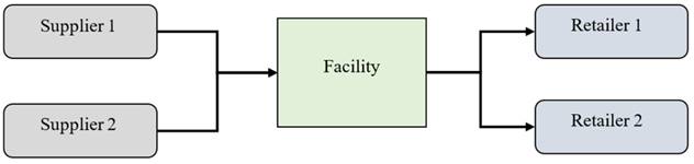
Table 1 shows an overview of some relevant research characteristics. Alashhab and Mlybari (2021), developed a model for multi-item SC design and planning. They have created a multi-item, multi-product, and multi-period mathematical model to maximize profit by optimizing supply, manufacturing, distribution, and inventory planning for a SC with two suppliers, one factory, and two retailers. In this proposed model, Xpress IVE was used to solve the issue, using Mixed Integer Linear Programming. Figure 1 shows the proposed SCN.

Figure 1

 

Figure 1 SCN

 

2. MODEL FORMULATION

The model involves the following sets, parameters, and variables:

Sets:

P: Set of products, mentioned by (p)

I: Set of items, mentioned by (i)

S: Set of prospective suppliers, mentioned by (s)

C: Set of prospective retailers, mentioned by (c)

T: Set of prospective, mentioned by (t)

 

Parameters:

Ff: the fixed cost in period (t)

DEMcpt: demand for retailer (c) of product (p) in period (t) (unit/ period)

REQip: Required amount of item (i) for product (p) (unit)

IIFp: the initial inventory of product (p) (unit)

FIFp: the final inventory of product (p) (unit)

Pct: the unit price of product (p) at retailer (c) in period (t) ($)

Wp: the weight of product (p) (kg)

Wi: the weight of items (i) (kg)

MHp: manufacturing hours for product (p) (hour)

Dsf: the linear distance between the supplier and the facility (km)

Dfc: the linear distance between the facility and the retailer (c) (km);

CAPsit: the capacity of supplier s for item (i) in period (t) (kg)

CAPHFt: Manufacturing capacity of the facility in period (t) (hour)

CAPMft: storage capacity for raw material of the facility in period (t)(kg)

CAPFSFt: Capacity of the storage facility in period (t) (kg)

MATCostsit: material cost per unit of item (i) supplied by supplier s in period (t) ($/kg)

MCft: manufacturing cost per hour for the facility in period (t) ($/hour)

NUCCf: non-utilized manufacturing capacity cost per hour of the facility ($/hour)

SCPUp: back-ordering cost per unit per period ($/unit/period)

HC: holding cost per unit weight per period in the facility store ($/kg/period)

Bsi: the batch size of the item (i) transported from the supplier to the factory (unit)

Bfp: batch size transported from the facility for product (p) to retailer (unit)

Tc: transport cost of the transport mode per kilometer in period (t) ($/km)

 

Variables:

Ls: If a supplier (s) is contracted, the binary variable is 1; otherwise, it will be 0.

Lsf: If a transportation link between supplier (s) and the factory is activated, a binary variable equal to 1 will be set.

Lfc: If a transportation link is activated between the factory and customer (c), the binary variable equals 1.

Qsfit: number of batches of item (i) transported from supplier (s) to the facility in period (t)

Qfcpt: number of batches of product (p) transported from the facility to retailer (c) in period (t)

Iffpt: number of batches transported from the facility to its store for product (p) in period (t)

Ifcpt: number of batches transported from store of the facility to retailer (c) for product (p) in period (t)

Rfpt: facility store a residual inventory of product (p) in period (t)

CSLc: Customer service level of customer (c)

M: is a big number

 

2.1. OBJECTIVE FUNCTIONS

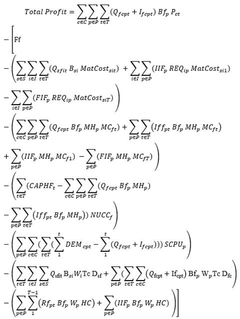
The objectives of this proposed model are to maximize profits, minimize total cost, and maximize OCSL. Equation 1, computes the profit by deducting the whole cost from the total revenue,

 

 

 

 

 

             Equation 1

                                                                             

2.1.1.  OVERALL CUSTOMER SERVICE LEVEL (OCSL)

Equation 2, computes the OCSL by summing all customers' customer service levels, as computed by.

 

                                   Equation 2

 

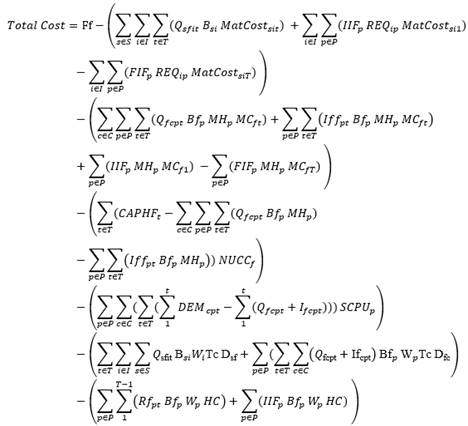
2.1.2.  TOTAL COST

Equation 3 shows the total cost including all fixed, material, manufacturing, and non-utilized capacity costs, as well as shortages, transportation, and inventory holding costs.

 

                  Equation 3

 

The material costs include all materials given to the factory by all suppliers, as well as the costs of the original inventory materials deducting the costs of the materials utilized to construct the final inventory that will be used after this planning time.

Production costs include manufacturing costs distributed to all retailers with the manufacturing costs of the initial inventory deducting used manufacturing costs of the final inventory after this planning time.

The cost of non-utilized capacity in facility is calculated by multiplying the depreciation per hour of machines during non-utilized time by the non-utilized capacity hours.

The shortage cost is determined by multiplying the shortage quantities of each product in all periods for all retailers by the shortage cost per unit for each period.

Transportation costs are also determined by multiplying the distance travelled by the transportation cost per unit of distance, for all shipments of all transportation modes in all periods for transporting raw materials from suppliers and finished goods to retailers.

Inventory costs, with exception of last period are calculated using the weights of residual product inventory at the end of each period and holding the initial inventory.

 

2.2. CONSTRAINTS

2.2.1.  BALANCE CONSTRAINTS

 

                                                                   Equation 4

 

                                        Equation 5

 

          Equation 6

 

                                                                                                   Equation 7

 

                                                                                    Equation 8

 

                                                                   Equation 9

                                                 Equation 10

 

Constraint Equation 4 to Equation 10 ensures the flow balancing of materials and products in the model.

 

2.2.2.  CAPACITY CONSTRAINTS

 

                                                                  Equation 11

 

                                                                   Equation 12

 

                Equation 13

 

                                                                         Equation 14

 

 Equation 11 ensures that a supplier total flow to the facility does not exceed the capacity of this supplier at each period.

 Equation 12 ensures that the total amount of material flowing into the facility from all sources does not exceed the facility's material capacity at each period.

Equation 13 ensures that total number of manufacturing hours for all manufactured and delivered products at the facility to each client and period do not exceed the manufacturing capacity hours.

 Equation 14 ensures that the residual inventory, during each period, does not exceed its capacity.

 

3. MODEL VERIFICATION

The effectiveness of model is clearly displayed in the following example.

 

3.1. VERIFICATION EXAMPLE INPUTS

In order to verify the model, two scenarios have been created. Table 2 tabulates the demands of each retailer of products over 6 periods for all scenarios.

Table 3 presents the weights of demands for each retailer of products over 6 periods for all scenarios. And Table 4 shows the demand for items needed to fulfil the demand for products. Finally, the list of other parameters and their respective values is given in Table 5.

 

Table 2

Table 2 Demand of retailers of products over 6 periods for all scenarios
Period	1	2	3	4	5	6
Scenario 1	500	1,000	3,000	2,500	2,000	1,500
Scenario 2	6000	4,000	4,000	500	500	500

 

Table 3

Table 3 Demand weight for all retailers of products over 6 periods for all scenarios
Scenario	Period	1	2	3	4	5	6
Scenario 1	Product 1	1500	3,000	9,000	7,500	6,000	4,500
	Product 2	2000	4,000	12,000	10,000	8,000	6,000
Scenario 2	Product 1	18000	12,000	12,000	1,500	1,500	1,500
	Product 2	24000	16,000	16,000	2,000	2,000	2,000

 

Table 4    

Table 4 Demand of items for all retailers of products over 6 periods for all scenarios
	Period	1	2	3	4	5	6
Scenario 1	Item 1	3000	6000	18000	15000	12000	9000
	Item 2	4000	8000	24000	20000	16000	12000
	Total Demand	7000	14000	42000	35000	28000	21000
Scenario 2	Item 1	36000	24000	24000	3000	3000	3000
	Item 2	48000	32000	32000	4000	4000	4000
	Total Demand	84000	56000	56000	7000	7000	7000

 

Table 5

Table 5 List of input parameters and their respective values
No.	Input parameter	Value	Unit	No.2	Input parameter3	Value4	Unit5
1	S and C	2	--	15	MCft	1	$/hr.
2	P and I	2	--	16	MHp	1, 2	hrs.
3	IIfp	0	Unit	17	MCft	10	$/hr.
4	FIfp	0	Unit	18	NUCCf	1	$/hr.
5	Pct	110, 220	$/Unit	19	SCPUp	5	$/period
6	WP 1,2	3, 4	Kg	20	HC	0.75	$/kg. period
7	MH 1,2	1, 2	Hrs	21	Bsi	1, 1	Unit
8	REQip	1, 2, 2, 2	Kg. /Unit	22	Bfp	1, 1	Unit
9	CAPHft	30,000	Hrs	23	TCt	0.05	$
10	CAPMft	50,000	Kg	24	Ff	50,000	$
11	CAPFSft	10,000	Kg	25	Bf	1	unit
12	MATCit	1, 1, 1, 1	$/kg	26	Dsf	55.8, 40.4	Km
13	CAPs1	9,000	Kg	27	Dfc	14.8, 22.4	Km
14	CAPs2	9,000	Kg	28	Wi	1	Kg

 

3.2. VERIFICATION EXAMPLES, RESULTS AND DISCUSSION

The following software and hardware are used to solve this model; Xpress IVE software on an Intel(R) Core (TM) i5-10210U CPU @ 1.60 GHz 2.10GHz (8 GB of RAM).

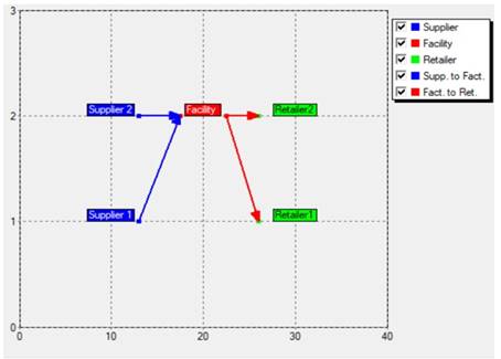
According to first scenario, the optimal network is shown in Figure 2, The demand was increasing and then descending. It is noticed also in the first and second periods, Figure 3, Figure 4 and Figure 5 that demand, and storage were fulfilled. The demand of third period was achieved from the actual production and residual storage. There was a shortage in the fourth period because item 2, Figure 5 was reached was at its highest possible capacity. In the fifth period, the previous shortage was recently compensated, finally the request was fulfilled.

Figure 2

                                                                         

Figure 2 The optimal network of the first scenario

 

Figure 3

                                                                         

Figure 3 Distribution by weights of the first scenario

 

Figure 4

                                                                         

Figure 4 Distribution weight of item 1 of the first scenario

 

Figure 5

                                                                         

Figure 5 Distribution weight of item 2 of the first scenario

 

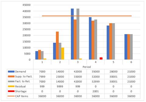
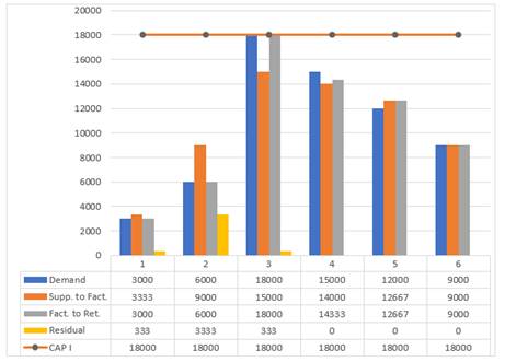
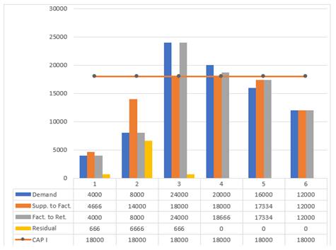
According to second scenario, the optimal network is shown in Figure 6 The demand of the first three perios are high as in Figure 7, Figure 8 and Figure 9 resulting in a shortage. The critical point of production was item 2, Figure 9, and production was at the highest limit from the first to the last period.

 

 

 

 

 

Figure 6

                                                                         

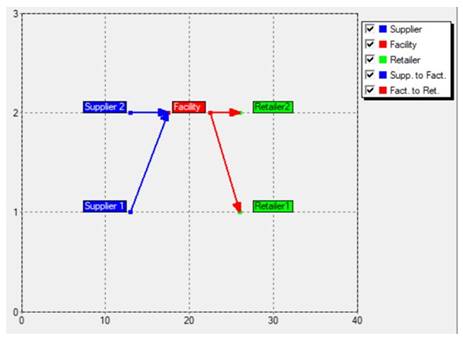
Figure 6 The resulted optimal network of the second scenario

 

Figure 7

                                                                         

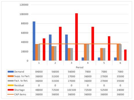
Figure 7 Distribution by weights of the second scenario

 

 

 

 

 

 

 

 

 

 

Figure 8

                                                                         

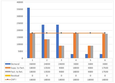
Figure 8 distribution weight of item 1 of the second scenario

 

Figure 9

                                                                         

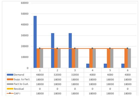
Figure 9  Distribution weight of item 2 of the second scenario

 

4. COMPUTATIONAL RESULTS AND ANALYSIS

In this section, the effect of changing the maximum allowable deviation on profit, OCSL, and total cost will be studied. Moreover, the effect of changing the objectives prioritization on the same factors will be also investigated. 

 

4.1. THE EFFECT OF CHANGING THE MAXIMUM ALLOWABLE DEVIATION

This study will measure the effect of the deviation from 0% to 50% with a step of 5% as shown in Table 6 on the first scenario according to the following optimization order (profit - total cost - OCSL), in the presence of shortage and residual.

 

Table 6

Table 6 Maximum allowed deviation
Maximum allowed deviation
	0	0.05	0.1	0.15	0.2	0.25
Profit	6069286	6050017	6029506	6002391	5978801	5955766
Total cost	860714	879983	900494	927609	951199	974234
Overall service level	100%	100%	100%	100%	100%	100%
Total revenue	6930000	6930000	6930000	6930000	6930000	6930000
Fixed cost	-50000	-50000	-50000	-50000	-50000	-50000
Material cost	-147000	-147000	-147000	-147000	-147000	-147000
Manufacturing cost	-63000	-63000	-63000	-63000	-63000	-63000
Nonutilized cost	-117000	-117000	-117000	-117000	-117000	-117000
Shortage cost	-3335	-3335	-21665	-45000	-65245	-78280
Transportation costs	-471381	-491400	-488705	-491198	-495506	-489731
Inventory holding cost	-8998	-8249	-13124	-14410	-13448	-29223
	0.3	0.35	0.4	0.45	0.5
Profit	5929999	5907612	5903262	5903262	5903262
Total cost	1000001	1022388	1026738	1026738	1026738
Overall service level	100%	100%	100%	100%	100%
Total revenue	6930000	6930000	6930000	6930000	6930000
Fixed cost	-50000	-50000	-50000	-50000	-50000
Material cost	-147000	-147000	-147000	-147000	-147000
Manufacturing cost	-63000	-63000	-63000	-63000	-63000
Nonutilized cost	-117000	-117000	-117000	-117000	-117000
Shortage cost	-99300	-109995	-114995	-114995	-114995
Transportation costs	-490705	-500896	-499870	-499870	-499870
Inventory holding cost	-32996	-34497	-34873	-34873	-34873

 

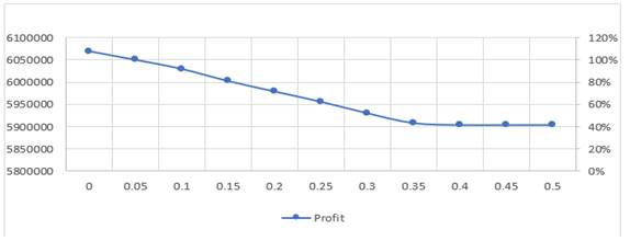
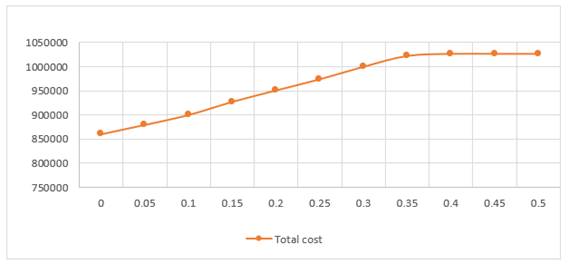
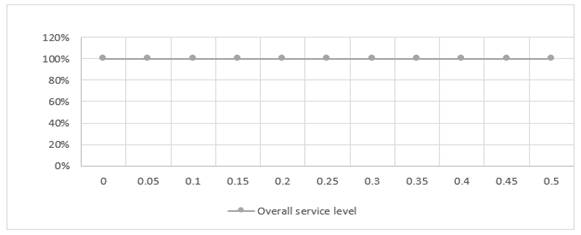
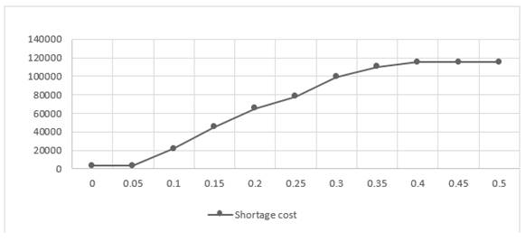
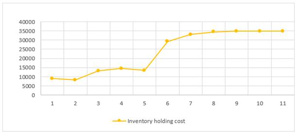
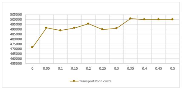
As noticed in, Table 6 the value of the OCSL, total revenue, fixed cost, material cost, manufacturing cost, and non-utilized cost are not changed with the change in deviation. The change occurred in the profit, total cost, transportation cost, shortage cost, and inventory holding cost are shown in Figure 10 to Figure 15

 

Figure 10

                                                                          

Figure 10 The effect of changing the Maximum allowable deviation on profit

 

Figure 11

                                                                         

Figure 11 The effect of changing the Maximum allowable deviation on total cost

 

Figure 12

                                                                          

Figure 12 The effect of changing the Maximum allowable deviation on overall service level

 

Figure 13

                                                                         

Figure 13 The effect of changing the Maximum allowable deviation on the shortage cost

 

 

 

Figure 14

                                                                         

Figure 14 The effect of changing the Maximum allowable deviation on the holding of inventory

 

Figure 15

                                                                         

Figure 15  The effect of changing the Maximum allowable deviation on transportation cost

 

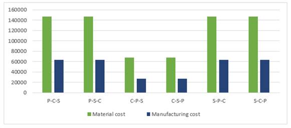
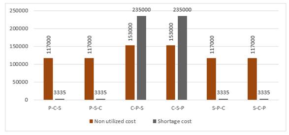
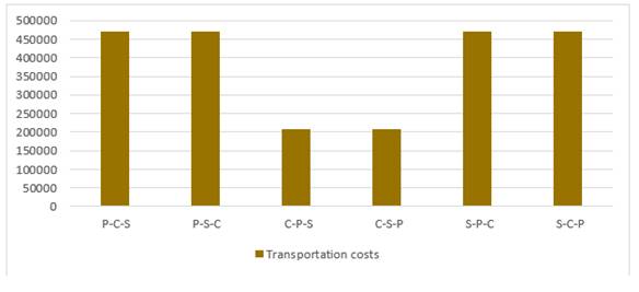
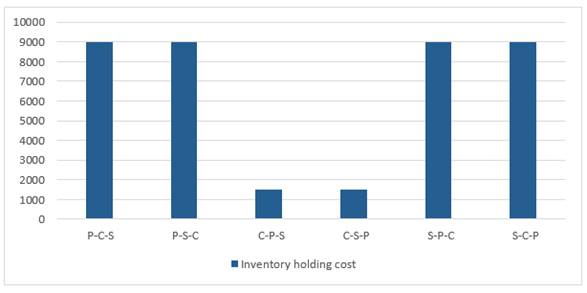
4.2. THE EFFECT OF CHANGING THE OBJECTIVES PRIORITIZATION

In this section, the effect of changing the objectives prioritization on profit, OCSL, and cost components will be studied.

 

Table 7

Table 7 Objectives prioritization
	Objective 1	Objective 2	Objective 3
Order 1 (P-C-S)	Profit	Total cost	OCSL
Order 2 (P-S-C)	Profit	OCSL	Total cost
Order 3 (C-P-S)	Total cost	Profit	OCSL
Order 4 (C-S-P)	Total cost	OCSL	Profit
Order 5 (S-P-C)	OCSL	Profit	Total cost
Order 6 (S-C-P)	OCSL	Total cost	Profit

 

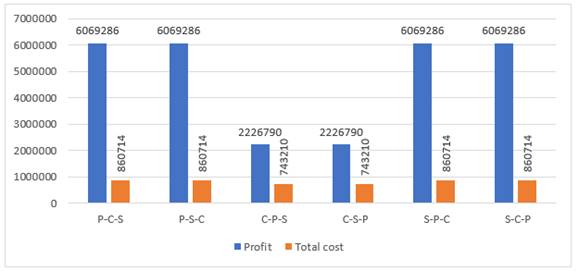
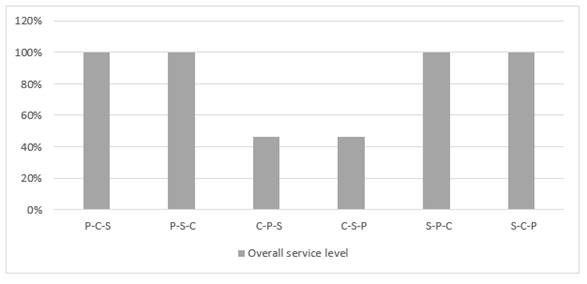
As shown in Figure 16 and Figure 17, both profit and OCSL maximum value have been achieved when giving and of them the first optimization priority as in the first, second, fifth and sixth orders because they are a non-conflicting objective.

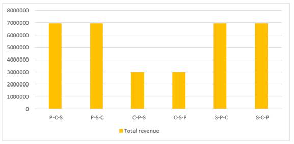
In the third and fourth oreders while the total cost is the main objective, the profit will be decreased compared to the other four orders. In the same aforementioned orders, total revenue, material cost, manufacturing cost, non-utilized, shortage transportation cost and inventory holding cost, have been decreased compared to the other four orders as shown in Figure 18 to Figure 22.

 

Figure 16

                                                                         

Figure 16 The effect of changing the objectives prioritization on profit and total cost

 

Figure 17

                                                                         

Figure 17 The effect of changing the objectives prioritization on OCSL

 

 

 

 

 

 

 

Figure 18

                                                                        

Figure 18  The effect of changing the objectives prioritization on total revenue

 

Figure 19

                                                                         

Figure 19 The effect of changing the objectives prioritization on material cost and manufacturing cost

 

Figure 20

                                                                        

Figure 20 The effect of changing the objectives prioritization on non-utilized cost and shortage cost

 

Figure 21

                                                                           

Figure 21  The effect of changing the objectives prioritization on transportation cost

 

Figure 22

                                                                         

Figure 22 The effect of changing the objectives prioritization on inventory holding

 

5. CONCLUSION

The developed multi-item, multi-product, and multi-period mathematical model has been successfully optimized for supply, production, distribution, and inventory planning for a multi-echelon SC of two suppliers, one factory, and two retailers, to maximize profit.

By solving and analysing the results of a thorough example, the efficiency has been demonstrated.

Supply chain performance has been investigated and analysed in terms of total revenue, cost, profit, and OCSL.

The model may be developed to:

1)     Study the impact of product quality on objectives, profit, total cost, and OCSL.

2)     Implement uncertainty of demand.

3)     Take the suppling disruption into account.

 

CONFLICT OF INTERESTS

None. 

 

ACKNOWLEDGMENTS

None.

 

REFERENCES

Al-Ashhab, M S. (2016). An optimization model for multi-period multi-product multi-objective production planning. International Journal of Engineering & Technology IJET-IJENS, 16(01).

Al-Ashhab, M. S. & Alanazi, F. (2022). Developing a multi-item, multi-product, and multi-period supply chain network design and planning model for perishable products. International Journal of Research - GRANTHAALAYAH, 10(4), 179-199.  https://doi.org/10.29121/granthaalayah.v10.i4.2022.4574

Al-Ashhab, M. S. & Fadag, H. (2018). Multi-Product Master Production Scheduling Optimization Modelling Using Mixed Integer Linear Programming And Genetic Algorithms. International Journal of Research-GRANTHAALAYAH, 6(5), 78-92. https://doi.org/10.29121/granthaalayah.v6.i5.2018.1429

Al-Ashhab, M. S. Afia, N. & Shihata, L. A. (2016). Objective Effect on the Performance of a Multi-Period Multi-Product Production Planning Optimization Model. International Journal of Mechanical & Mechatronics Engineering IJMME-IJENS, 16(03), 13.

Al-Ashhab, M.S. Attia, T. & Munshi, S. M. (2017). Multi-Objective Production Planning Using Lexicographic Procedure. American Journal of Operations Research, 7(03), 174.  https://doi.org/10.4236/ajor.2017.73012 

Al-e-hashem, S. M. J. M. & Rekik, Y. (2014). Multi-product multi-period Inventory Routing Problem with a transshipment option : A green approach. International Journal of Production Economics, 157, 80-88. https://doi.org/10.1016/j.ijpe.2013.09.005

Alashhab, M. S. & Mlybari, E. A. (2021). Developing a multi-item, multi-product, and multi-period supply chain planning optimization model. Indian Journal of Science and Technology, 14(37), 2850-2859. https://doi.org/10.17485/IJST/v14i37.867

Alashhab, M.S. & Mlybari, E. A. (2020). Developing a robust green supply chain planning optimization model considering potential risks. GEOMATE Journal, 19(73), 208-215. https://doi.org/10.21660/2020.73.52896

Altiparmak, F. Gen, M. Lin, L. & Paksoy, T. (2006). A genetic algorithm approach for multi-objective optimization of supply chain networks. Computers & Industrial Engineering, 51(1), 196-215. https://doi.org/10.1016/j.cie.2006.07.011

Aramyan, L. H. Lansink, A. G. J. M. O. Van Der Vorst, J. G. A. J. & Van Kooten, O. (2007). Performance measurement in agri‐food supply chains: a case study. Supply Chain Management : An International Journal. https://doi.org/10.1108/13598540710759826

Axsäter, S. (2015). Inventory control (225). Springer. https://doi.org/10.1007/978-3-319-15729-0

Folan, P. & Browne, J. (2005). A review of performance measurement: Towards performance management. Computers in Industry, 56(7), 663-680. https://doi.org/10.1016/j.compind.2005.03.001

Franca, R. B. Jones, E. C., Richards, C. N. & Carlson, J. P. (2010). Multi-objective stochastic supply chain modeling to evaluate tradeoffs between profit and quality. International Journal of Production Economics, 127(2), 292-299. https://doi.org/10.1016/j.ijpe.2009.09.005

Ganeshan, R. (1999). Managing supply chain inventories : A multiple retailer, one warehouse, multiple supplier model. International Journal of Production Economics, 59(1-3), 341-354. https://doi.org/10.1016/S0925-5273(98)00115-7

Guillén, G. Mele, F. D. Bagajewicz, M. J. Espuna, A. & Puigjaner, L. (2005). Multiobjective supply chain design under uncertainty. Chemical Engineering Science, 60(6), 1535-1553. https://doi.org/10.1016/j.ces.2004.10.023

Gunasekaran, A. & Kobu, B. (2007). Performance measures and metrics in logistics and supply chain management : a review of recent literature (1995-2004) for research and applications. International Journal of Production Research, 45(12), 2819-2840. https://doi.org/10.1080/00207540600806513

Hadi, S. & Parubak, B. (2016). Supply Chain Operational Capability Affecting Business Performance of Creative Industries. 2016 Global Conference on Business, Management and Entrepreneurship, 212-216. https://doi.org/10.2991/gcbme-16.2016.39

Jang, Y.-J. Jang, S.-Y. Chang, B.-M. & Park, J. (2002). A combined model of network design and production/distribution planning for a supply network. Computers & Industrial Engineering, 43(1-2), 263-281. https://doi.org/10.1016/S0360-8352(02)00074-8

Jindal, A. Sangwan, K. S. & Saxena, S. (2015). Network design and optimization for multi-product, multi-time, multi-echelon closed-loop supply chain under uncertainty. Procedia Cirp, 29, 656-661. https://doi.org/10.1016/j.procir.2015.01.024

Kotler, P. & Keller, K. L. (2016). A framework for marketing management. Pearson Boston, MA.

Mangun, N. Rombe, E. Taqwa, E. Sutomo, M. & Hadi, S. (2021). Ahp Structure For Determining Sustainable Performance Of Indonesian Seafood Supply Chain From Stakeholders Perspective. Journal of Management Information and Decision Sciences, 24(7), 1-10.

Mentzer, J. T. DeWitt, W. Keebler, J. S. Min, S., Nix, N. W. Smith, C. D. & Zacharia, Z. G. (2001). Defining supply chain management. Journal of Business Logistics, 22(2), 1-25.  https://doi.org/10.1002/j.2158-1592.2001.tb00001.x

Mohamed, S. & Naji Aldosari. (2022). Modelling and Solving a Sustainable, Robust Multi-Period Supply Chain Network for Perishable Products. INDIAN JOURNAL OF ENGINEERING, 19(51), 184-195.  

Morash, E. A. (2001). Supply chain strategies, capabilities, and performance. Transportation Journal, 37-54.

Muslimin, P. B. Muhammad, N. & Suryadi, H. (2017). The Impact of marketing and supply chain operational capabilities on business performance in Indonesian creative industry. International Journal of Economic Research, 14(12).

Pasandideh, S. H. R. Niaki, S. T. A. & Asadi, K. (2015). Bi-objective optimization of a multi-product multi-period three-echelon supply chain problem under uncertain environments : NSGA-II and NRGA. Information Sciences, 292, 57-74. https://doi.org/10.1016/j.ins.2014.08.068

Riswanto, A. (2021). Competitive intensity, innovation capability and dynamic marketing capabilities. Research Horizon, 1(1), 7-15. https://doi.org/10.54518/rh.1.1.2021.7-15

Rombe, E. & Hadi, S. (2022). The impact of supply chain capability and supply chain performance on marketing performance of retail sectors. Uncertain Supply Chain Management, 10(2), 593-600. https://doi.org/10.5267/j.uscm.2021.11.005

Vrat, P. (2014). Materials management. Springer Texts in Business and Economics, 978-981. https://doi.org/10.1007/978-81-322-1970-5

Wang, F., Lai, X., & Shi, N. (2011). A multi-objective optimization for green supply chain network design. Decision Support Systems, 51(2), 262-269.  https://doi.org/10.1016/j.dss.2010.11.020

Yan, H. Yu, Z. & Cheng, T. C. E. (2003). A strategic model for supply chain design with logical constraints: formulation and solution. Computers & Operations Research, 30(14), 2135-2155. https://doi.org/10.1016/S0305-0548(02)00127-2