
|
|
|
|
A VENDOR-BUYER SUPPLY CHAIN MODEL WITH IMPERFECT PRODUCTION UNDER TIME, PRICE AND PRODUCT RELIABILITY DEPENDENT DEMANDBiswarup Samanta 1 1, 3, 4 Department of Mathematics, Jadavpur University, Kolkata,700032, India2 Regent Engineering College, Barrackpore, Kolkata 700121, India |
|
||
|
|
|||
|
Received 20 September 2021 Accepted 01 October 2021 Published 22 October 2021 Corresponding Author Biswarup
Samanta, biswarupsamanta6@gmail.com DOI 10.29121/ijetmr.v8.i10.2021.1046 Funding:
This
research received no specific grant from any funding agency in the public,
commercial, or not-for-profit sectors. Copyright:
© 2021
The Author(s). This is an open access article distributed under the terms of
the Creative Commons Attribution License, which permits unrestricted use, distribution,
and reproduction in any medium, provided the original author and source are
credited.
|
ABSTRACT |
|
|
|
This
article investigates a single-vendor single-buyer supply chain model where
the market demand depends on time as well as selling price and product
reliability. The vendor’s production rate is not constant but depends on the
market demand. The vendor’s production process is not perfectly reliable; it
may produce some percentage of defective items during a production run. The
vendor takes up a lot-for-lot policy for delivering the ordered quantity to
the buyer who performs 100% screening after receiving each lot. The average
total profit of the integrated supply chain is derived and a numerical
example is taken to validate the developed model. The optimal results of the
proposed model are also discussed for some particular cases. Sensitivity
analysis is performed to investigate the influence of key model-parameters on
the optimal results. |
|
||
|
Keywords: Supplychain; Vendor; Buyer; Pricing; Reliability; Imperfect Production 1. INTRODUTION Over the past several
decades, the integration of the individual mind-sets of the vendor and the
buyer into the supply chain has been a matter of curiosity to many supply
chain researchers. This helps to identify problem areas in the process,
allows businesses to take decisive steps and reduce costs to improve on final
prices. Improving end-customer gratification and reliability is a by-product
of an integrated supply chain as customer’s perception improves on-time
delivery. The integrated policy makes the supply chain more transparent,
making buyers and vendors more flexible and progressive in relation to each
other and to the market. Undoubtedly the market demand plays a vital role in
determination of such an integrated policy. There are many products
for which the market demand may increase with the passage of time. However,
there are many other factors like product price, after sales service,
advertisement, product quality, etc. which can also affect the market demand.
When a customer wants to buy a product from a shopping mall or supermarket,
two things are knocked in his/her mind. What is the price of the product? How
reliable the product is? Price and reliability play important roles in the
minds of strong customers while buying a product like mobile phone or laptop.
Apple is outstanding for its superior quality but it is so expensive that it
always remains beyond the reach of the middle class family. It only
influences high class customers. On the other hand, Samsung |
|
||


and Lenovo are famous for products that reach relatively low prices and features. Consumer’s preference for higher prices to quality will influence himself to buy Apple products which are regarded suitable for their requirements. By preferring features and prices, end-customers’ accommodate on product quality and buy Samsung or Lenovo products. The vendors need both advanced manufacturing processes and good quality raw materials if they want to produce high reliability products. To assemble laptops, Lenovo uses low cost raw-materials to reduce overall costs whereas Apple uses very high quality ingredients in MacBooks and hence overall costs increases. To optimize a firm’s profit, a balance needs to be struck between time, price and reliability of its product.
Integrated supply chain
models have been developed in the literature based on some limited assumptions.
One of these assumptions is that the vendor produces products of perfect
quality. In fact, there can be a few imperfect items in any production lot due
to poor control of processes, non-adherence to plans, inappropriate operating
guidelines, and so on. If the vendor has to pay extra cost for each defective
item produced then it is profitable to reduce the number of defective items in
the production process. The rate of defective items produced by the vendor
affects other critical decisions such as the vendor’s production lot size and
reliability of the product. Further, a vendor has a reputation for making more
reliable product which is preferable for a buyer to place an order. To improve
the quality of a product, investment can be made to reduce errors in the
vendor’s production process. In an integrated supply chain system, when
non-conformable items are produced, it is most likely that some kind of
supervision/inspection activity needs to be performed by the buyer before
selling the goods to the end customers.
This article develops an
integrated single-vendor single-buyer supply chain model with time, price and
reliability dependent market demand. The vendor’s production process is
imperfect and it rejects all the non-conformable items produced during a
production run. The buyer screens all the items before selling to
end-customers. The defective items are sold in the secondary market with a
discount. The vendor plans for a lot-for-lot production policy to meet the
buyer’s demand. The primary objectives of this article are to find the response
of the following queries:
1)
How much time
will be taken by the vendor and the buyer to produce a lot and sell to
customers?
2)
How much time
will be delayed by the vendor to produce items ordered by the buyer?
3)
What will be the
selling price of each good item from the buyer’s side?
4)
What will be the
reliability of a product produced by the vendor?
The rest of the paper is
arranged as follows: In the next section, the related literatures are reviewed.
Section 3 presents assumptions and notations for developing the proposed model.
Section 4 discusses the mathematical model and solution procedure. A numerical
example is provided in Section 5. The optimal results are analyzed in Section
6. Section 7 concludes the paper and indicates some future research
directions.
2.
LITERATURE REVIEW
In reality, the market
demand of certain products may not remain constant always; it may change with
the passage of time. Hariga and Benkherouf (1994) presented a heuristic inventory model in which the
market demand changes exponentially in time over a finite planning horizon. Hariga (1996) developed an inventory lot-sizing model with time-varying demand for
deteriorating items. An inventory model with Weibull deterioration, time
proportional demand rate and effects of inflation was developed by Chen (1998). Khanra and Chaudhuri (2003) proposed an inventory model with quadratic time dependent demand where
the on-hand inventory deteriorates with time. Ghosh and
Chaudhuri (2006) developed this model by considering shortages in inventory. Actually, a
large volume of research papers on time dependent demand are available in the
literature Giri and Maiti
(2012), Chowdhury et al. (2014), Samanta
et al. (2018)
Now-a-days the
customer’s demand depends not only on time but also on other factors such as
product price, after sales service, advertisement, product quality, etc. Price
of a product plays an important role in customer’s mind. So, it is more
realistic to include price sensitive demand. Burwell et al.
(1991) determined the optimal lot size and selling price when a supplier offers
all-unit quantity discounts by considering price-dependent demand and allowing
for shortages. A finite period system was considered by Datta and Paul (2001) under multi-replenishment scenario, where the demand rate is influenced
by both displayed stock level and selling price. An economic production
quantity (EPQ) model for deteriorating items was developed by Teng and Chang (2005) where the demand rate depends on the selling price and display stock
level with limited display space consideration. You (2005) investigated a supply chain model in which a leading member of the supply
chain gets the scope to settle value of the product to impress demand and more
revenues. Avinadav et al. (2013) formulated a model for finding the optimal pricing, order quantity and
replenishment period for deteriorating items with price- and time-dependent
demand. Yang et
al. (2013) studied a piecewise production-inventory model for a deteriorating item
with time-varying and price-sensitive demand to optimize the vendor’s total
profit. Herbon
and Khmelnitsky (2017) considered a dynamic pricing policy for perishable products, attracting
customers to buy less-fresh products due to expiry, potentially increasing
revenue and eliminating waste. Numerous works in this direction could be found
in the literature You and Hsieh
(2007), Chen et
al. (2010), Ghosh et
al. (2011), Kim et
al. (2011), Bhunia and Shaikh
(2014), Maiti
and Giri (2015), Giri and
Roy (2015), Maiti
and Giri (2017), Chan (2019), Roy and
Giri (2020).
When end-customers buy
some goods from buyers, it is the outcome of the endeavors of several members
of supply chains. But, the main credit goes to the vendor as the customer
prefer that product for his reliability. So, the balance between price and
reliability is an important factor in inventory/supply chain management.
Therefore, the reliability of a product must be taken into consideration. An
EPQ model with a flexible and imperfect production process was proposed by Cheng (1989) under reliability consideration. Sadjadi et al. (2009) considered a production-marketing problem where the reliability of the
production process assumed to be imperfect and the inventory and the setup
costs per production cycle are not known in advance. An inventory model with
imperfect production process was developed by Shah and Shah (2014) for time-declining demand pattern where reliability of the production
process was considered as a decision variable. Shah and Vaghela (2018) analysed EPQ model with time and advertisement sensitive demand with the
effect of inflation and reliability.
The above works
considered reliability of the product and its effect on the optimal results.
However, none of these works would consider the market demand as a function of
reliability of the product. Khara et al. (2017) considered a model that deals with an imperfect production process, where
both perfect and imperfect quality items are produced and demand depends on
selling price and reliability of the product. Later, Khara et al. (2019) developed that model by considering demand as a function of selling
price, reliability of the product and advertisement cost. Shah and Naik (2020) investigated an inventory model with imperfect production process and
reliability-dependent demand.
Chung
and Wee (2008) developed an integrated production-inventory deteriorating model
considering imperfect production, inspection planning and warranty-period-and
stock-level-dependant demand. Jauhari (2016) proposed a vendor-buyer model where the lot transferred from the vendor
to the buyer contains some defective items and the buyer conducts an imperfect
inspection process to classify the quality of the items. Jauhari et al.
(2016) developed an imperfect production-inventory model where the buyer uses
periodic review policy to manage his inventory. The demand on the buyer side
was assumed to be normally distributed, and the shortage was assumed to be
fully backordered and the defective rate of the items was assumed to be fixed.
In this article, we
consider the market demand as a function of time, selling price and reliability
of the product. The production rate is not constant but depends on the market
demand, as considered by Giri and
Maiti (2012). The variable production rate was also considered by Jauhari et al.
(2016). In the literature, unit production cost is considered as a fixed. But in
reality, it should depends on order quantity to be produced by the vendor. More
production implies less unit production cost and less production implies
expensive production cost. On the other hand, if a vendor prefers to produce an
item with more reliable to keep/increase his reputation in market, then (s)he
has to use raw material which are also more reliable. Thus the material cost
depends on reliability of the product. The demand may change at any time during
production process. In that case, to maintain the on-time delivery to the
buyer, the vendor’s production rate has to be changed. Therefore, we consider
the unit production cost as a function of material cost and production rate.
Variable unit production cost was also considered in different forms by Khara et al. (2017).
3. MODEL ASSUMPTIONS AND NOTATIONS
The notations used
throughout the paper are as follows:
|
|
: |
time interval between successive deliveries
(decision variable) |
|
|
: |
time delayed by the vendor to start
production (decision variable) |
|
|
: |
unit selling price for the buyer(decision
variable) |
|
|
: |
reliability of the product (decision
variable) |
|
|
: |
variable time |
|
|
: |
number of cycles |
|
|
: |
demand rate at the buyer |
|
|
: |
production rate at the vendor |
|
|
: |
scaling constant for production rate |
|
|
: |
set up cost per production run for the
vendor |
|
|
: |
ordering cost per order for the buyer |
|
|
: |
unit stock-holding cost per unit per unit
time for the vendor |
|
|
: |
unit stock-holding cost per unit per unit
time for the buyer |
|
|
: |
quantity produced by the vendor during the
period |
|
|
: |
market demand during the period |
|
|
: |
material cost |
|
|
: |
price elasticity to demand |
|
|
: |
reliability elasticity to demand |
|
|
: |
reliability elasticity to material cost |
|
|
: |
fixed material cost |
|
|
: |
material cost increases the reliability of
the produced item |
|
|
: |
variation constant of tool/die costs |
|
|
: |
transportation cost per shipment |
|
|
: |
unit production cost |
|
|
: |
screening rate |
|
|
: |
unit screening cost |
|
|
: |
unit wholesale price for the vendor |
|
|
: |
discount price per defective item for the
vendor |
|
|
: |
buyer’s inventory level |
|
|
: |
vendor’s inventory level |
|
|
: |
buyer’s profit function |
|
|
: |
vendor’s profit function |
|
|
: |
average total profit to the whole supply
chain |
The following
assumptions are made to develop the proposed integrated vendor-buyer inventory
model:
·
The supply chain
consists of a single-vendor and a single-buyer who stocks and sells a single
product.
·
The demand for a
product depends on time ![]() selling price
selling price ![]() as well as the
reliability of the product
as well as the
reliability of the product ![]() . We assume that the demand rate
. We assume that the demand rate ![]() and
and ![]() are real
constants. This type of demand was considered by Khara et al. (2017).
are real
constants. This type of demand was considered by Khara et al. (2017).
·
The vendor
follows the lot-for-lot policy for replenishment made to the buyer.
·
The buyer
receives the first order from the vendor at time ![]() and (s)he
receives order from the vendor in every
and (s)he
receives order from the vendor in every ![]() time interval.
time interval.
·
Shortages are not
allowed in the buyer’s inventory.
·
As the
reliability of the product depends not only on the manufacturing system but
also on the quality of the raw material of the product, we assume that the
material cost ![]() is an
increasing function of the reliability (
is an
increasing function of the reliability (![]() ) of the product such that
) of the product such that ![]() where
where ![]() and
and ![]() .
.
·
The production
rate of the vendor varies with the demand rate. Also, the production rate is
greater than the demand rate. We take the production rate ![]() as
as ![]() where
where ![]() .
.
·
As the vendor’s
production rate is greater than the buyer’s demand rate, the vendor may start
production with a time delay ![]() in the n-th
production cycle.
in the n-th
production cycle.
·
The production
cost not only depends on the material cost ![]() but also on
tool or die cost, which is proportional to the vendor’s production rate.
Therefore, the unit production cost
but also on
tool or die cost, which is proportional to the vendor’s production rate.
Therefore, the unit production cost ![]() is assumed as
is assumed as ![]() where
where ![]() .
.
·
The vendor’s
production process is not perfectly reliable. During a production run, it may
produce some defective (non-conforming) items.
·
The buyer starts
error-free screening after received products from vendor. We assume that the
number of perfect units is at least equal to the demand during the screening
time.
·
Product quality
may be imperfect. In other words, only ![]() of all produced
items meet the demand while
of all produced
items meet the demand while ![]() of items are
defective. It is apparent that the maximum reliability of the production
process cannot exceed
of items are
defective. It is apparent that the maximum reliability of the production
process cannot exceed ![]() . This type of assumption was also considered by Sadjadi et al.
(2009).
. This type of assumption was also considered by Sadjadi et al.
(2009).
·
The vendor
produced ![]() quantity in
total during n-th production cycle
and delivered to the buyer to meet the customer / market demand
quantity in
total during n-th production cycle
and delivered to the buyer to meet the customer / market demand ![]() in the next
cycle.
in the next
cycle.
4. MODEL FORMULATION
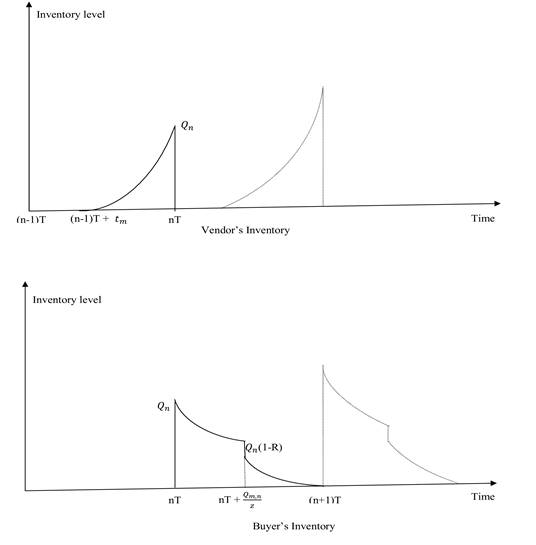
The graphical
presentation of the vendor-buyer model is shown in Figure 1. We suppose that ![]() is the length
of each cycle. For the
is the length
of each cycle. For the ![]() -th cycle, the vendor starts his/her production at
time
-th cycle, the vendor starts his/her production at
time ![]() and the buyer
receives his/her order of quantity
and the buyer
receives his/her order of quantity ![]() from the vendor
at time
from the vendor
at time ![]() ,
, ![]() and meets the
market demand
and meets the
market demand ![]() for period
for period ![]() . The buyer starts screening at a rate of
. The buyer starts screening at a rate of ![]() units per unit
time immediately after receiving the products from the buyer. The buyer’s
screening is completed at time
units per unit
time immediately after receiving the products from the buyer. The buyer’s
screening is completed at time ![]() . We assume that only
. We assume that only ![]() of received
products are acceptable as good products to meet the customer demand. The
customer’s demand rate at time
of received
products are acceptable as good products to meet the customer demand. The
customer’s demand rate at time ![]() is
is ![]() where
where ![]() and
and ![]() are real
constants.
are real
constants.
Therefore, the total
demand during the period ![]() is given by
is given by
![]() (1)
(1)
|
|
|
Figure 1 A
schematic diagram to represent the vendor’s and the buyer’s inventory. |
The quantity ![]() produced by the
vendor in the time interval
produced by the
vendor in the time interval ![]() is given by
is given by
![]()
![]() (2)
(2)
4.1. DECENTRALISED MODEL
4.1.1. VENDOR’S PERSPECTIVE
Let ![]() be the vendor’s
inventory level at any time
be the vendor’s
inventory level at any time ![]() . Then the instantaneous states of the vendor’s
inventory level can be described by the differential equation:
. Then the instantaneous states of the vendor’s
inventory level can be described by the differential equation:
![]() (3)
(3)
Solving (3), we get
![]() (4)
(4)
At time ![]() , we have
, we have
![]()
![]()
The vendor’s holding cost per unit time for
the period ![]()
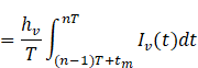
![]()
The vendor’s production cost per unit time in
that period
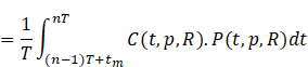
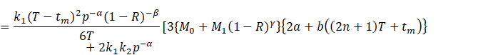
![]()
As the vendor’s sales revenue = ![]() set-up cost
set-up cost ![]() , discount cost for defective items per unit time =
, discount cost for defective items per unit time = ![]() , therefore, the vendor’s total profit per unit time
is given by
, therefore, the vendor’s total profit per unit time
is given by
![]()
![]()
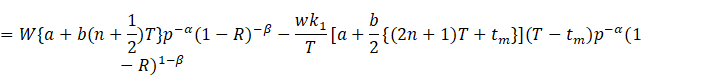

![]() (5)
(5)
4.1.2. BUYER’S PERSPECTIVE
The differential
equation governing the buyer’s inventory level at any time ![]() is given by
is given by
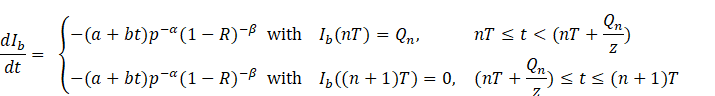
Solving, we get
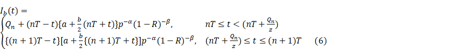
From (6), the buyer’s
inventory level at the time point![]() is given by
is given by
![]() (7)
(7)
Also, we have
![]() (8)
(8)
From (7) and (8), we
have
![]() (9)
(9)
Which is a quadratic
equation in ![]() with
discriminant
with
discriminant
![]() .
.
Hence there always
exists a positive (real) production lot size ![]() of the vendor
in any time interval
of the vendor
in any time interval ![]() , for all
, for all ![]() .
.
Now, the buyer’s holding
cost per unit time
![]()
![]()
![]()
![]()
Also, sales revenue per
unit time = ![]() , purchase cost per unit time =
, purchase cost per unit time =![]() , transportation cost per unit time =
, transportation cost per unit time = ![]() , screening cost per unit time =
, screening cost per unit time = ![]() and ordering
cost per unit time =
and ordering
cost per unit time = ![]() . Therefore, the buyer’s total profit per unit time is
given by
. Therefore, the buyer’s total profit per unit time is
given by
![]()
![]()
![]()
![]() (10)
(10)
Proposition 1 When the
buyer’s selling price ![]() is known, the profit function
is known, the profit function ![]() is concave with respect to
is concave with respect to ![]() for all
for all ![]() where
where
![]()
![]()
![]()
provided that ![]()
Proof.
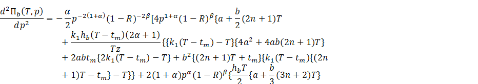
Differentiating (10) twice with respect to ![]() , we get
, we get
![]()
It is clear from the
above that ![]() provided that
provided that
![]() which gives
which gives ![]() (say)
(say)
![]() which gives
which gives
![]()
or, ![]() (say)
(say)
![]()
or, ![]()
or, ![]() [since
[since ![]() ]
]
or, ![]()
or, ![]() (say)
(say)
Hence the proposition is
proved.
Proposition 2 For ![]() where
where ![]() and
and
![]() , the profit function
, the profit function ![]() is concave with respect to
is concave with respect to ![]() for all
for all ![]() satisfying the condition
satisfying the condition ![]()
Proof.
Differentiating (10) twice with respect to ![]() , we get
, we get
![]()
From above, ![]() provided that
the following conditions hold:
provided that
the following conditions hold:
![]() which implies
which implies ![]() .
.
![]()
Considering the above
inequation as equation, we see that the two roots of the equation are
We take ![]() such that
such that![]() .
.
![]()
As the buyer’s selling
price ![]() is always
greater than the vendor’s wholesale price
is always
greater than the vendor’s wholesale price ![]() , we have
, we have ![]() . Hence, the proposition is proved.
. Hence, the proposition is proved.
Proposition 3 For known ![]() ,
, ![]() and
and ![]() , the vendor’s profit
function
, the vendor’s profit
function ![]() is concave with respect to
is concave with respect to ![]() if
if ![]() provided
that
provided
that ![]() .
.
Proof.
Differentiating (5) twice with respect to ![]() , we get
, we get

Clearly, ![]() if
if ![]()
![]()
![]()
![]()
If ![]() , then from above we have,
, then from above we have,
![]()
Again, if ![]() , then from above we have,
, then from above we have,
![]()
This proves the
proposition.
Proposition 4 For known ![]() , the profit function
, the profit function ![]() is concave with respect to
is concave with respect to ![]() for all
for all ![]() where,
where, ![]() and
and ![]() .
.
Proof.
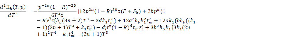
Differentiating (5) twice with respect to ![]() , we get
, we get
![]()
![]()
Clearly, the profit
function ![]() will be concave
with respect to
will be concave
with respect to ![]() if the
following two conditions are satisfied:
if the
following two conditions are satisfied:
![]()
![]()
From ![]() we have
we have![]()
From ![]() we have
we have![]()
Hence, the proposition
is proved.
4.2. CENTRALISED MODEL
The average total profit
of the integrated supply chain is given by
![]()
![]()
![]()
![]()
![]()
![]()
![]() (11)
(11)
Proposition 5 In case of the
centralized supply chain system, the product reliability ![]() depends on the decision variables
depends on the decision variables ![]() and
and ![]() given by the
relation
given by the
relation
![]() (12)
(12)
Proof.
The vendor delivers ![]() quantity of
items to the buyer, of which
quantity of
items to the buyer, of which ![]() is found to be
defective after completion of the buyer’s screening process. Hence, only
is found to be
defective after completion of the buyer’s screening process. Hence, only ![]() quantity is
considered as good items and sold by the buyer to meet the market demand
quantity is
considered as good items and sold by the buyer to meet the market demand ![]() . Since, there is no shortage and no excess items, we
can claim that
. Since, there is no shortage and no excess items, we
can claim that ![]() Using (1) and
(2), we have
Using (1) and
(2), we have
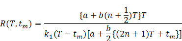
Proposition 6 The buyer’s
selling price ![]() depends on the decision variables
depends on the decision variables ![]() and
and ![]() given by the
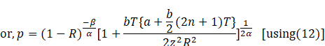
relation
given by the
relation ![]() (13)
(13)
where ![]() is given by (12).
is given by (12).
Proof.
Substituting the value of ![]() from (2) into
the relation (9), we get
from (2) into
the relation (9), we get
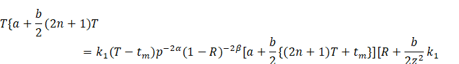
![]()
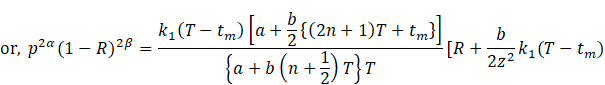
![]()
Hence, the proposition
is proved.
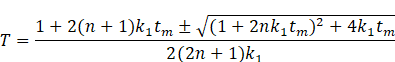
Proposition 7 To meet the customer demand ![]() , the vendor produces
, the vendor produces ![]() quantity of
items with delay in time
quantity of
items with delay in time ![]() satisfying the
relation
satisfying the
relation
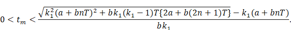
Proof. Since ![]() , therefore, from (12) it is obvious that
, therefore, from (12) it is obvious that ![]() .
.
Again, ![]() gives
gives![]()
or, ![]()
Considering the above
inequation as equation, we see that the two roots of the equation are
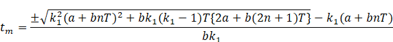
The smaller root is
negative and hence the proposition is proved.
Using (12) and (13), the
profit function ![]() can be reduced
to the function
can be reduced
to the function ![]() of two
independent variables
of two
independent variables ![]() and
and ![]() . It is not possible to prove analytically that
. It is not possible to prove analytically that ![]() is jointly
concave. However, we can prove the following proposition:
is jointly
concave. However, we can prove the following proposition:
Proposition 8 For known
values of ![]() and
and ![]() , the profit function
, the profit function ![]() is concave with respect to
is concave with respect to ![]() for all
for all ![]() according as
according as ![]() and
and ![]() satisfies the relation
satisfies the relation ![]() where,
where,
![]()
![]()
![]()
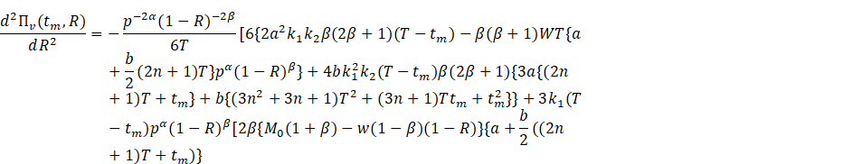
Proof.
Differentiating (11) twice with respect to ![]() , we get
, we get
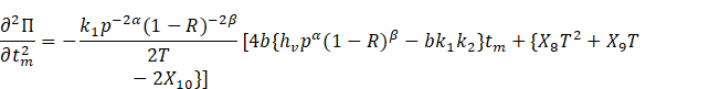
The profit function ![]() will be concave
with respect to
will be concave
with respect to ![]() if
if
![]()
For ![]() , we have
, we have![]() .
.
Since the vendor’s
production delay time ![]() is always
positive, the numerator of the right hand expression must be positive and hence
is always
positive, the numerator of the right hand expression must be positive and hence
![]() . This proves the proposition.
. This proves the proposition.
Proposition 9 For pre-defined
values of ![]() and
and ![]() , the profit function
, the profit function ![]() is concave with respect to
is concave with respect to ![]() if
if
![]()
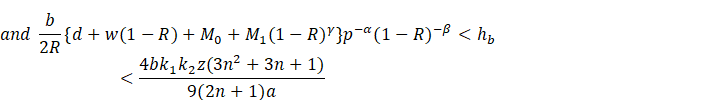
Proof.
Differentiating (11) twice with respect to ![]() , we have
, we have
![]()
![]()
![]()
![]()
![]()
![]()
In the right-hand side
of the above equation, the expression within the third bracket will be positive
if the following three conditions are satisfied:
![]()
![]()
![]()
From ![]() we have,
we have, ![]() .
.
From ![]() we have,
we have, ![]() provided that
provided that ![]()
From ![]() we have
we have ![]() .
.
Hence, the proposition
is proved.
5. NUMERICAL EXAMPLE
To illustrate the
developed models numerically, we consider the following data-set (Giri and Maiti (2012)):
![]() and
and ![]() . Also, we consider
. Also, we consider ![]() in appropriate
units.
in appropriate
units.
To check the concavity
of the profit function ![]() , we observe that
, we observe that ![]() and
and ![]() have to satisfy
the conditions
have to satisfy
the conditions![]() and the variable
and the variable ![]() has no
restriction. So, we consider
has no
restriction. So, we consider ![]() and
and ![]() The decision
variables
The decision
variables![]() and
and ![]() are found from the propositions 6 and 7, respectively
as
are found from the propositions 6 and 7, respectively
as ![]() and
and ![]() . Then we have,
. Then we have, ![]() and the
determinant of Hessian matrix associate with
and the
determinant of Hessian matrix associate with ![]() is given by
is given by
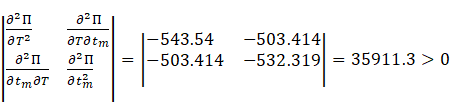
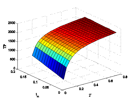
This proves that, for
the above data set, the profit function ![]() is concave in
is concave in ![]() and
and ![]() . One evidence is shown in Figure 2 for
. One evidence is shown in Figure 2 for ![]() . We observe that, if we move from one cycle to the
next cycle, the buyer’s ordering time period
. We observe that, if we move from one cycle to the
next cycle, the buyer’s ordering time period ![]() and the
vendor’s delay time
and the
vendor’s delay time ![]() to start
production change very slowly whereas the average total profit of the supply
chain increases considerably. Without any loss of generality, we consider the
sixth cycle
to start
production change very slowly whereas the average total profit of the supply
chain increases considerably. Without any loss of generality, we consider the
sixth cycle ![]() and we obtain
and we obtain ![]() and
and ![]() . In this sixth cycle, the vendor produces
. In this sixth cycle, the vendor produces ![]() quantity of
items. After receiving these items, the buyer performs screening and
quantity of
items. After receiving these items, the buyer performs screening and ![]() of
of ![]() quantity of
items is considered as good quality and perfect items to meet the demand
quantity of
items is considered as good quality and perfect items to meet the demand ![]() given by
(1).
given by
(1).
|
|
|
Figure 2 Graphical
representation of the profit function |
The buyer’s selling
price ![]() , the product reliability
, the product reliability ![]() and the average
total profit of the supply chain increase as we move from one cycle to the next
cycle. Since the changes in
and the average
total profit of the supply chain increase as we move from one cycle to the next
cycle. Since the changes in![]() and
and![]() are
insensitive, we present in Table 1 the values of
are
insensitive, we present in Table 1 the values of ![]() and
and ![]() for successive
ten cycles.
for successive
ten cycles.
|
Table 1 Optimal results of the proposed model for successive ten
cycles |
|||
|
|
|
|
|
|
1 |
12.9386 |
0.874390 |
2035.33 |
|
2 |
12.9523 |
0.837046 |
2053.32 |
|
3 |
12.9660 |
0.837050 |
2071.32 |
|
4 |
12.9798 |
0.837055 |
2089.34 |
|
5 |
12.9935 |
0.837059 |
2107.37 |
|
6 |
13.0073 |
0.837063 |
2125.42 |
|
7 |
13.0210 |
0.837068 |
2143.48 |
|
8 |
13.0348 |
0.837072 |
2161.56 |
|
9 |
13.0485 |
0.837076 |
2179.66 |
|
10 |
13.0623 |
0.837080 |
2197.77 |
5.1. THE CASE OF
![]()
In this scenario, we
assume that the demand rate depends on time only and hence we put ![]() and
and ![]() in our proposed
model. The demand rate becomes
in our proposed
model. The demand rate becomes ![]() and the
vendor’s production rate is
and the
vendor’s production rate is ![]() with
with ![]() Also, we assume
that unit production cost does not depend on reliability and it is fixed and
denoted by
Also, we assume
that unit production cost does not depend on reliability and it is fixed and
denoted by ![]() . To compare the results with the optimal results of
our proposed model, we take
. To compare the results with the optimal results of
our proposed model, we take ![]() ,
, ![]() and
and ![]() . This
. This
|
Table 2 Comparison of the results of our model and the model with |
|||||
|
|
Model with |
Our model |
Difference of profits |
||
|
|
|
|
|
|
|
|
1 |
3.19089 |
1.06363 |
1016.77 |
2035.33 |
1018.56 |
|
2 |
4.10970 |
1.36990 |
1052.09 |
2053.32 |
1001.23 |
|
3 |
4.91770 |
1.63923 |
1092.64 |
2071.32 |
978.68 |
|
4 |
5.32066 |
1.77355 |
1134.25 |
2089.34 |
955.09 |
|
5 |
5.44683 |
1.81561 |
1174.16 |
2107.37 |
933.21 |
|
6 |
5.43545 |
1.81182 |
1211.56 |
2125.42 |
913.86 |
|
7 |
5.35954 |
1.78651 |
1246.45 |
2143.48 |
897.03 |
|
8 |
5.25452 |
1.75151 |
1279.06 |
2161.56 |
882.50 |
|
9 |
5.13785 |
1.71262 |
1309.67 |
2179.60 |
869.93 |
|
10 |
5.01832 |
1.67277 |
1338.52 |
2197.77 |
859.25 |
implies that ![]() of received
items from the vendor is sold by the buyer at the retail price
of received
items from the vendor is sold by the buyer at the retail price ![]() to meet the
market demand. All the remaining assumptions are kept unchanged. Thus, we take
to meet the
market demand. All the remaining assumptions are kept unchanged. Thus, we take ![]() ,
, ![]() and
and ![]() and all other
parameter-values are same as assumed before. With this data-set, we find that
for
and all other
parameter-values are same as assumed before. With this data-set, we find that
for ![]() ,
, ![]() and the average
total profit of the supply chain as
and the average
total profit of the supply chain as ![]() which is
$2125.42 less than that of our proposed model. In Table 2, we compare the optimal results of ten successive
cycles with those of the proposed model.
which is
$2125.42 less than that of our proposed model. In Table 2, we compare the optimal results of ten successive
cycles with those of the proposed model.
5.2. THE CASE OF
![]()
Here we assume that the
vendor’s produced items are all perfect, although in reality it may not always
happen. To compare the results with those of the proposed model, we assume the
market
|
Table 3 Comparison of profits of the proposed model and our model
with |
|||||
|
Model with |
Our model |
Difference of profits |
|||
|
|
|
|
|
|
|
|
1 |
4.10977 |
1.36992 |
729.98 |
2035.33 |
1305.35 |
|
2 |
5.99780 |
1.99927 |
765.33 |
2053.32 |
1287.99 |
|
3 |
8.86478 |
2.95493 |
815.01 |
2071.32 |
1256.31 |
|
4 |
11.4611 |
3.82038 |
878.73 |
2089.34 |
1210.61 |
|
5 |
13.3829 |
4.46097 |
951.72 |
2107.37 |
1155.65 |
|
6 |
14.7948 |
4.93159 |
1030.37 |
2125.42 |
1095.05 |
|
7 |
15.8619 |
5.28731 |
1112.63 |
2143.48 |
1030.85 |
|
8 |
16.6930 |
5.56433 |
1197.30 |
2161.56 |
964.26 |
|
9 |
17.3571 |
5.78570 |
1283.65 |
2179.60 |
895.95 |
|
10 |
17.8994 |
5.96648 |
1371.22 |
2197.77 |
826.55 |
demand as ![]() , where
, where ![]() and
and ![]() . The production rate is
. The production rate is ![]() with
with ![]() In this case,
the buyer’s holding cost changes to
In this case,
the buyer’s holding cost changes to ![]() . As before, we assume that unit production cost
. As before, we assume that unit production cost ![]() . Since, all products are perfect, there is no need to
screen and hence we take
. Since, all products are perfect, there is no need to
screen and hence we take ![]() and
and ![]() . All the remaining assumptions are kept unchanged.
Thus, in numerical data, we take
. All the remaining assumptions are kept unchanged.
Thus, in numerical data, we take ![]() ,
, ![]() and
and ![]() , keeping all other parameter-values unchanged. From
the numerical experiment, we find that
, keeping all other parameter-values unchanged. From
the numerical experiment, we find that ![]() ,
, ![]() and the average
total profit of the supply chain model is
and the average
total profit of the supply chain model is ![]() , which is
, which is ![]() less than that
of our proposed model. In Table 3, we compare the optimal results of ten successive
cycles with those of our proposed model.
less than that
of our proposed model. In Table 3, we compare the optimal results of ten successive
cycles with those of our proposed model.
6. SENSITIVITY ANALYSIS
In this section, we
investigate the effect of change of one parameter-value at a time keeping the
remaining parameter-values unchanged. The sensitivity of the parameters ![]() and
and ![]() are shown in
the Figure 3, Figure 4, Figure 5, Figure 6, Figure 7. Some insights from our investigation are given
below.
are shown in
the Figure 3, Figure 4, Figure 5, Figure 6, Figure 7. Some insights from our investigation are given
below.
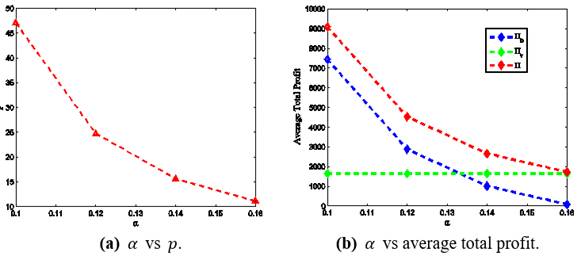
1) Both the buyer’s selling price ![]() and the product
reliability
and the product
reliability ![]() increase
rapidly as
increase
rapidly as ![]() increases (Figure 3
increases (Figure 3![]() ). The vendor has to produce more reliable product as
). The vendor has to produce more reliable product as ![]() increases. As a
result, the vendor’s unit production cost increases and at the same time, the
market
increases. As a
result, the vendor’s unit production cost increases and at the same time, the
market
|
|
|
Figure 3 Change
(%) in optimal results w.r.t. |
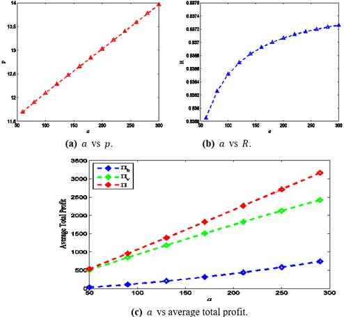
demand also increases. Therefore, the buyer’s average total
profit as well as the vendor’s average total profit increase as ![]() increases.
Consequently the average total profit of the integrated supply chain increases
as
increases.
Consequently the average total profit of the integrated supply chain increases
as ![]() increases (Figure 3
increases (Figure 3 ![]() ).
).
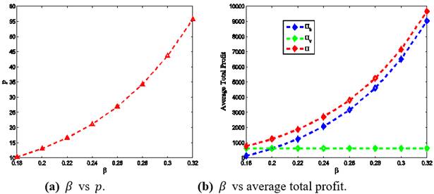
2) As ![]() increases, the
selling price
increases, the
selling price ![]() increases but
the rate of increase in
increases but
the rate of increase in ![]() is not so high.
The buyer’s average total profit increases significantly but the vendor’s
average total profit increase is very low. As a result, the average total
profit of the integrated supply chain model increases moderately as the value
of
is not so high.
The buyer’s average total profit increases significantly but the vendor’s
average total profit increase is very low. As a result, the average total
profit of the integrated supply chain model increases moderately as the value
of ![]() increases (Figure 4
increases (Figure 4 ![]() ).
).
|
|
|
Figure 4 Change (%) in
optimal results w.r.t. |
3) The product reliability ![]() is not affected
by the price elasticity to demand
is not affected
by the price elasticity to demand ![]() but the buyer’s
selling price is highly sensitive with respect to
but the buyer’s
selling price is highly sensitive with respect to ![]() as shown in Figure 5
as shown in Figure 5![]() . A
. A ![]() increase in the
value of
increase in the
value of ![]() results
results ![]() decrease in the
value of the selling price
decrease in the
value of the selling price ![]() . But it does not have any impact on the vendor’s
average total profit. A lower selling price results in lower profit from the
buyer’s perspective as well as from the integrated supply chain’s perspective (Figure 5
. But it does not have any impact on the vendor’s
average total profit. A lower selling price results in lower profit from the
buyer’s perspective as well as from the integrated supply chain’s perspective (Figure 5 ![]() ).
).
|
|
|
Figure 5 Change (%) in
optimal results w.r.t. |
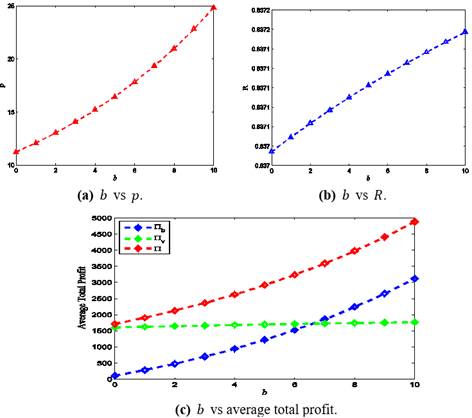
4) As ![]() increases, the
selling price
increases, the
selling price ![]() and the average
total profits of the buyer and the entire supply chain increase (Figure 6
and the average
total profits of the buyer and the entire supply chain increase (Figure 6![]() ).
).
|
|
|
Figure 6 Change (%) in
optimal results w.r.t. |
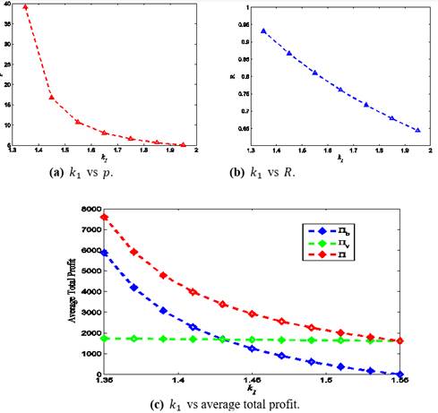
5) Figure 7![]() shows that, as
shows that, as ![]() increases, the
buyer’s selling price and reliability of the product decrease (Figure 7
increases, the
buyer’s selling price and reliability of the product decrease (Figure 7![]() ). Due to increase in production rate, the vendor’s
production time decreases but there is at most no change in the average total
profit of the vendor. However, the average total profit of integrated supply
chain decreases as
). Due to increase in production rate, the vendor’s
production time decreases but there is at most no change in the average total
profit of the vendor. However, the average total profit of integrated supply
chain decreases as ![]() increases (Figure 7
increases (Figure 7![]() ).
).
|
|
|
Figure 7 Change
(%) in optimal results w.r.t. |
7. CONCLUSION
The paper considers a
single vendor single buyer integrated supply chain model in which the market
demand is assumed to be dependent on time, price and reliability of the
product. The vendor follows a lot-for-lot policy. The items are delivered to
the buyer with an agreement that the buyer himself screens all those products
and, if any item is found defective, it should be sold with price discount and
the cost must be borne by the vendor. The reputation of the vendor and the
buyer increase as the product bears good and perfect quality to the best of
their knowledge. On the other hand, the end customer’s satisfaction increases
as the product is more reliable. In this paper, some propositions are derived
which help to choose the data-set in the numerical example as well as to find
the optimal values of the decision variables. From the numerical analysis, we
have found that the vendor has to maintain the reliability of the product and
produce items not more ![]() defective. It
is also observed that the scaling constant
defective. It
is also observed that the scaling constant ![]() for the demand
act important roles to increase the profits of the buyer, vendor and the integrated
supply chain.
for the demand
act important roles to increase the profits of the buyer, vendor and the integrated
supply chain.
In this article, we have
assumed a deterministic market demand, which has limited applications in the
business world. So, this model can be extended by considering stochastic
demand. Shortages are not allowed in our model. So, one can extend the present
model with inclusion of shortage in the buyer’s inventory. One can also
consider multi-vendor and/or multi-buyer supply chain for further study. Terms
and conditions may be imposed by the vendor to sell the defective items (from
buyer’s screening) with price discount.
REFERENCES
A Bhunia and A Shaikh (2014). A deterministic inventory model for deteriorating items with selling price dependent demand and three-parameter Weibull distributed deterioration. International Journal of Industrial Engineering Computations, 5(3):497-510. Retrieved from https://doi.org/10.5267/j.ijiec.2014.2.002
Avi Herbon and Eugene Khmelnitsky (2017). Optimal dynamic pricing and ordering of a perishable product under additive effects of price and time on demand. European Journal of Operational Research, 260(2): 546-556. Retrieved from https://doi.org/10.1016/j.ejor.2016.12.033
B Samanta, Bibhas C Giri, and K S Chaudhuri (2018). A Vendor-Buyer Supply Chain Model for Deteriorating Item with Quadratic Time-Varying Demand and Pro-rata Warranty Policy. In International workshop of Mathematical Analysis and Applications in Modeling, pages 371-383. Springer. Retrieved from https://doi.org/10.1007/978-981-15-0422-8_31
Balaji Roy and Bibhas C Giri (2020). A three-echelon supply chain model with price and two-level quality dependent demand. RAIRO-Operations Research, 54(1):37-52. Retrieved from https://doi.org/10.1051/ro/2018066
Barun Khara, Jayanta Kumar Dey, and Shyamal Kumar Mondal (2017). An inventory model under development cost-dependent imperfect production and reliability-dependent demand. Journal of Management Analytics, 4(3):258-275. Retrieved from https://doi.org/10.1080/23270012.2017.1344939
Barun Khara, Jayanta Kumar Dey, and Shyamal Kumar Mondal (2019). Effects of product reliability dependent demand in an EPQ model considering partially imperfect production. International Journal of Mathematics in Operational Research, 15(2):242-264. Retrieved from https://doi.org/10.1504/IJMOR.2019.10022969
Bibhas C Giri and B Roy (2015). A single-manufacturer multi-buyer supply chain inventory model with controllable lead time and price-sensitive demand. Journal of Industrial and Production Engineering, 32(8):516-527. Retrieved from https://doi.org/10.1080/21681015.2015.1086442
Bibhas C Giri and T Maiti (2012). Supply chain model for a deteriorating product with time-varying demand and production rate. Journal of the Operational Research Society, 63(5): 665-673. Retrieved from https://doi.org/10.1057/jors.2011.54
C J Chung and H-M Wee (2008). An integrated production-inventory deteriorating model for pricing policy considering imperfect production, inspection planning and warranty-period-and stock-level-dependant demand. International Journal of Systems Science, 39(8):823-837. Retrieved from https://doi.org/10.1080/00207720801902598
Haoya Chen, Youhua Frank Chen, Chun-Hung Chiu, Tsan-Ming Choi, and Suresh Sethi (2010). Coordination mechanism for the supply chain with leadtime consideration and price-dependent demand. European Journal of Operational Research, 203(1):70-80. Retrieved from https://doi.org/10.1016/j.ejor.2009.07.002
Hau-Ling Chan (2019). Supply chain coordination with inventory and pricing decisions. International Journal of Inventory Research, 5(3):234-250. Retrieved from https://doi.org/10.1504/IJIR.2019.10020307
Jen-Ming Chen (1998). An inventory model for deteriorating items with time-proportional demand and shortages under inflation and time discounting. International Journal of Production Economics, 55(1):21-30. Retrieved from https://doi.org/10.1016/S0925-5273(98)00011-5
Jinn-Tsair Teng and Chun-Tao Chang (2005). Economic production quantity models for deteriorating items with price-and stock-dependent demand. Computers & Operations Research, 32(2):297-308. Retrieved from https://doi.org/10.1016/S0305-0548(03)00237-5
Jungkyu Kim, Yushin Hong, and Taebok Kim (2011). Pricing and ordering policies for price-dependent demand in a supply chain of a single retailer and a single manufacturer. International Journal of Systems Science, 42(1):81-89. Retrieved from https://doi.org/10.1080/00207720903470122
Moncer A Hariga and Lakdere Benkherouf (1994). Optimal and heuristic inventory replenishment models for deteriorating items with exponential time-varying demand. European Journal of Operational Research, 79(1):123-137. Retrieved from https://doi.org/10.1016/0377-2217(94)90400-6
Moncer Hariga (1996). Optimal EOQ models for deteriorating items with time-varying demand. Journal of the Operational Research Society, 47(10):1228-1246. Retrieved from https://doi.org/10.1057/jors.1996.151
Nita H Shah and Bhavin J Shah (2014). EPQ model for time-declining demand with imperfect production process under inflationary conditions and reliability. International Journal of Operations Research, 11(3):91-99.
Nita H Shah and Chetansinh R Vaghela (2018). Imperfect production inventory model for time and effort dependent demand under inflation and maximum reliability. International Journal of Systems Science: Operations & Logistics, 5(1):60-68. Retrieved from https://doi.org/10.1080/23302674.2016.1229076
Nita H Shah and Monika K Naik (2020). Inventory Policies with Development Cost for Imperfect Production and Price-Stock Reliability-Dependent Demand. In Optimization and Inventory Management, pages 119-136. Springer. Retrieved from https://doi.org/10.1007/978-981-13-9698-4_7
P S You (2005). Inventory policy for products with price and time-dependent demands. Journal of the Operational Research Society, 56(7):870-873, Retrieved from https://doi.org/10.1057/palgrave.jors.2601905
Peng-Sheng You and Yi-Chih Hsieh (2007). An EOQ model with stock and price sensitive demand. Mathematical and Computer Modelling, 45(7-8):933-942. Retrieved from https://doi.org/10.1016/j.mcm.2006.09.003
Po-Chung Yang, Hui-Ming Wee, Shen-Lian Chung, and Yong-Yan Huang (2013). Pricing and replenishment strategy for a multi-market deteriorating product with time-varying and price-sensitive demand. Journal of Industrial & Management Optimization, 9(4):769. Retrieved from https://doi.org/10.3934/jimo.2013.9.769
R Roy Chowdhury, S K Ghosh, and K S Chaudhuri (2014). An order-level inventory model for a deteriorating item with time-quadratic demand and time-dependent partial backlogging with shortages in all cycles. American Journal of Mathematical and Management Sciences, 33(2):75-97. Retrieved from https://doi.org/10.1080/01966324.2014.881173
S K Ghosh and K S Chaudhuri (2006). An EOQ model with a quadratic demand, time-proportional deterioration and shortages in all cycles.International Journal of Systems Science, 37(10):663-672. Retrieved from https://doi.org/10.1080/00207720600568145
S K Ghosh, Sudhansu Khanra, and K S Chaudhuri (2011). Optimal price and lot size determination for a perishable product under conditions of finite production, partial backordering and lost sale. Applied Mathematics and Computation, 217(13):6047-6053. Retrieved from https://doi.org/10.1016/j.amc.2010.12.050
Seyed J Sadjadi, Mir-Bahador Aryanezhad, and Armin Jabbarzadeh (2009). An integrated pricing and lot sizing model with reliability consideration. In 2009 International Conference on Computers & Industrial Engineering, pages 808-813. IEEE. Retrieved from https://doi.org/10.1109/ICCIE.2009.5223880
Sudhansu Khanra and K S Chaudhuri (2003). A note on an order-level inventory model for a deteriorating item with time-dependent quadratic demand. Computers & Operations Research, 30(12):1901-1916. Retrieved from https://doi.org/10.1016/S0305-0548(02)00113-2
TCE Cheng (1989). An economic production quantity model with flexibility and reliability considerations. European Journal of Operational Research, 39(2):174-179. Retrieved from https://doi.org/10.1016/0377-2217(89)90190-2
Tal Avinadav, Avi Herbon, and Uriel Spiegel (2013). Optimal inventory policy for a perishable item with demand function sensitive to price and time. International Journal of Production Economics, 144(2):497-506. Retrieved from https://doi.org/10.1016/j.ijpe.2013.03.022
Tapan Kumar Datta and Karabi Paul (2001). An inventory system with stock-dependent, price-sensitive demand rate. Production planning \& control, 12(1):13-20. Retrieved from https://doi.org/10.1080/09537280150203933
Tarun Maiti and Bibhas C Giri (2015). A closed loop supply chain under retail price and product quality dependent demand. Journal of Manufacturing Systems, 37:624-637. Retrieved from https://doi.org/10.1016/j.jmsy.2014.09.009
Tarun Maiti and Bibhas C Giri (2017). Two-period pricing and decision strategies in a two-echelon supply chain under price-dependent demand. Applied Mathematical Modelling, 42:655-674. Retrieved from https://doi.org/10.1016/j.apm.2016.10.051
Timothy H Burwell, Dinesh S Dave, Kathy E Fitzpatrick, and Melvin R Roy (1991). An inventory model with planned shortages and price dependent demand.Decision Sciences, 22(5):1187-1191. Retrieved from https://doi.org/10.1111/j.1540-5915.1991.tb01916.x
Wakhid Ahmad Jauhari, Nelita Putri Sejati, and Cucuk Nur Rosyidi (2016). A collaborative supply chain inventory model with defective items, adjusted production rate and variable lead time. International Journal of Procurement Management, 9(6):733-750. Retrieved from https://doi.org/10.1504/IJPM.2016.10000438
Wakhid Ahmad Jauhari (2016). Integrated vendor-buyer model with defective items, inspection error and stochastic demand. International Journal of Mathematics in Operational Research, 8(3):342-359. Retrieved from https://doi.org/10.1504/IJMOR.2016.075520
|
|
 This work is licensed under a: Creative Commons Attribution 4.0 International License
© IJETMR 2014-2021. All Rights Reserved.