data sample points.  Literature [Uddin et al. (2019)] proposed a hyperspectral dimension reduction method based on Segmented Principal Component Analysis (SPCA).  Literature [Jayaprakash et al. (2020)] proposed a hyperspectral dimension reduction method based on Linear Discriminant Analysis (LDA)

However, these classical subspace learning methods cannot obtain low-dimensional manifold structures embedded in high-dimensional data.  Recent studies show that there are often embedded nonlinear low-dimensional manifold structures in high-dimensional data.  Manifold learning has become a very effective method for dimensionality reduction of hyperspectral images. Its representative methods include isometric Mapping (ISOMAP).  Laplacian Eigenmaps (LE) and Locally Linear Embedding (LLE), etc. [Wan et al. (2017), Dongyang and Li (2018)].  

However, these nonlinear methods can only reduce the dimension of the training sample set.  To solve this problem, He proposed Local Preserving Projection (LPP) and Neighborhood Preserving Embedding (NPE) algorithms to extend LE and LLE respectively [Qiao et  (2010)], so that the manifold learning method can be extended to the test sample set [ Kianisarkaleh and Ghassemian (2016),  Zhai et al. (2016), Gao et al. (2016)].  

In recent years, sparse representation can adaptively describe the reconstructed relationship between data.  Representative methods include Sparsity Preserving Projections (SPP) [Qiao et  (2010)] and Manifold Sparsity Preserving Projections (MSPP)[Tabejamaat and Mousavi (2017)]. SPP aims to keep the sparse reconstruction relationship of data by minimizing the objective function related to L1 regularization.  The resulting projection is not affected by rotation, reordering, and translation of the data.  Compared with LPP and NPE methods, SPP can automatically select its neighborhood, which is more convenient in practical application.  

Based on existing research [Uddin et al. (2019), Jayaprakash et al. (2020), Wan et al. (2017), Dongyang and Li (2018), Qiao et  (2010),  Kianisarkaleh and Ghassemian (2016),  Zhai et al. (2016), Gao et al. (2016), Wang et al. (2017), Lv  et al. (2017), Tabejamaat and Mousavi (2017), Dong et al. (2021), Yc (2021), Yuan  (2021)], this paper proposes a hyperspectral image classification method based on Manifold Data Analysis and Sparse Subspace Projection (MDASSP).  Good results have been achieved in small samples.  In this method, the sparse coefficient matrix is established by L1 regularization, and the sparse subspace projection of the original data is obtained by solving an optimization problem.  The correlation of the original data is preserved in low dimensional space. To keep the manifold geometry structure of the original data, the manifold learning method is introduced to regularize the objective function.  Experiments on real hyperspectral data sets show that the new method can improve the classification accuracy under small samples.

 

2.     Manifold data analysis and sparse subspace projection method

In the hyperspectral image classification problem, the training sample set is expressed as: . Wherein,  is the number of sample points, and the dimension of sample points is . is the corresponding category information, is the category number. The purpose of dimensionality reduction is to find a projection matrixand convert the original data of dimension  into projection data of dimension  ().  The conversion formula is: . Where,  is the dimension reduction vector corresponding to the sample point . In the new sample space, the classifier trains and classifies dimensionality reduction vectors.

Sparse Representation [Hairong and Turgay (2018)] is also called Sparse Coding.  The aim is to express most or all of the original signals with a linear combination of fewer basic signals.  The opposite concept of sparse representation is dense representation.  The dense representation sample can be transformed into the appropriate sparse representation by finding the appropriate dictionary for the sample points of the dense representation.  Thus, the classification and recognition task can be simplified, and the model complexity is also reduced.  The sparse representation method in this paper uses the remaining sample points in the dataset to reconstruct the given sample points.  Sparsity ensures that most of the reconstruction coefficients are zero, and only a few coefficients related to a given sample point are non-zero.  The sparse coefficient can reflect the correlation between sample points.  

Given a pixel sample point , Sparse representation method uses  to refactoring .  This problem can be translated into the following optimization problem:  

                                                         (1)

Wherein, is a  dimensional vector

 used to represent the reconstruction coefficient of the sample point .  norm is used to ensure the sparsity of coefficients.  However, regularization problem is a NP hard problem.  Therefore, regularization is used to approximately replace regularization, so the optimization problem becomes:  

                                                         (2)

The optimization problem of regularization can be solved by LARS algorithm [Efron et al. (2004)].  For each sample point , LARS algorithm can be used to calculate the corresponding reconstruction coefficient .  Therefore, a sparse coefficient matrix can be constructed.  

Sparse coefficient matrix describes the correlation between original sample points.  The purpose of sparse subspace projection is to find a projection matrix .  This matrix can transform the  dimension vector of the original space into dimension vector (), while ensuring the invariable correlation between sample points.  The solving process is transformed into an optimization problem, which is expressed as follows:  

                             (3)

Wherein, is the projection matrix.  The optimization objective function can be derived as follows:  

                       (4)

Wherein,  is the identity matrix of  order. . In order to avoid degradation, constraint conditions are added.

Therefore, the optimization problem becomes the following form:

                                                           (5)

In order to maintain the manifold geometry structure of the data, a manifold learning method is introduced to regularize the objective function:  

                              (6)

Wherein, is the similarity matrix.  The manifold regular term can be derived as follows:  

Therefore, the optimization problem becomes the following form:

                                                           (7)

Wherein, .                                      

The optimization problem is equivalent to the generalized feature decomposition problem as follows:

                                                        (8)

The projection vector  in the objective function of optimization problem (7) corresponds to the eigenvector corresponding to the jth eigenvalue of generalized eigendecomposition problem (8).  Therefore, the eigenvectors  corresponding to the smallest q eigenvalues after generalized eigendecomposition constitute the solution of optimization problem (7).

 

3.     RESULTS AND DISCUSSIONS

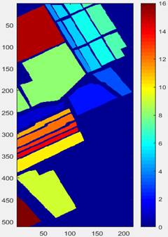
In order to verify the effectiveness of hyperspectral image classification method based on manifold data analysis and sparse subspace projection (MDASSP), experiments are carried out on real hyperspectral data sets.  Salinas data set was collected by AVIRIS sensor located over Salinas Valley in California, USA.  The original data contains 224 band images, of which band 108-112, 154-167, and band 224th cannot be reflected by water and are generally not used.  We have 204 bands left.  The spatial resolution of the dataset is 3.7m.  The size of the image is 512×217.  It therefore contains 111,104 pixels in total.  Among them, 56,975 pixels are background pixels and 54,129 pixels can be applied to classification.  These pixels are grouped into a total of 16 categories including Fallow, Celery, etc.

Figure 1(a) is the pseudo-color image generated by the superposition of the two-dimensional matrix of three bands (1,50,150) extracted as three channels of RGB image.  Figure 1 (b) is its real ground object annotation map.  There are a total of 16 feature categories (as shown in Table 1).  The values are integers 1 to 16, and the integer 0 represents the background.  The color corresponding to each feature category is shown on the vertical bar to the right of Figure 1 (b).

(a)    Pseudo-color map Figure 1 Salinas dataset	(b) Ground truth map

        

The preprocessing of the dataset consists of two steps: first, remove the noise bands that cannot be reflected by water, and then normalize the data.  After preprocessing, the labeled sample points were randomly divided into training set and test set.  The training set is used to learn the projection matrix of lower dimensional space.  All test set sample points are mapped to low-dimensional space by projection matrix, and then classified in low-dimensional space by nearest neighbor classifier.  In order to evaluate the performance of different algorithms, the experiment was repeated 20 times with randomly selected training sets, and finally the average classification accuracy of each method was obtained.  

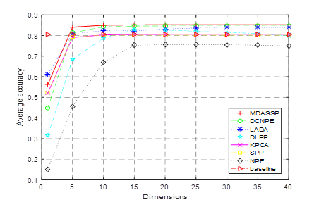
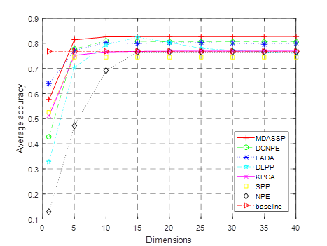
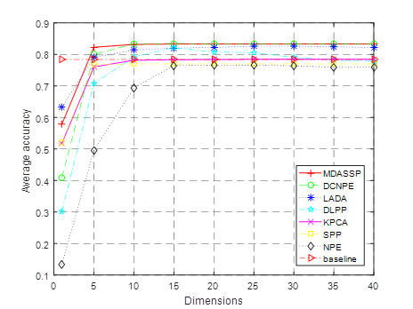
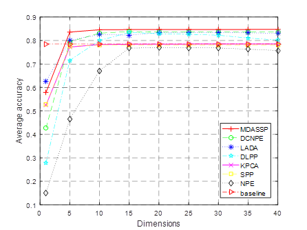
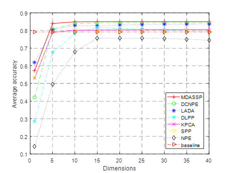
DCNPE method in literature [Lv et al. (2017)], LADA method in literature [Wang et al. (2017)], DLPP method in literature [Deng et al. (2015)], Kernel Principal Component Analysis (KPCA for short), sparse preserving projection (SPP for short) and domain-preserving embedding (NPE for short) are selected and compared with MDASSP method.  For better comparison, the parameters of each method are adjusted to the best.  In order to demonstrate the classification effect of the new method in the case of small samples, 3~7 labeled sample points were randomly selected from each class to form the training set.  The comparison of classification accuracy of various methods in different training sets is shown in Figure 2 .  

(a)i=3

(b)i=4

(c)i=5

 

(d)i=6

(e)i=7

Figure 2 Comparisons of average classification accuracy of Salinas dataset

 

In this experiment, i (i =3,4,5,6,7) marked sample points were randomly selected from each ground feature category to form the training set.  The remaining sample points constitute the test set.  The training set is used to learn the projection matrix of low dimensional space.  The test set is first projected into low dimensional space by matrix and then classified and identified.  Subgraphs (a)~(e) of Figure 2 respectively correspond to the average classification accuracy curves of different dimensionality reduction methods after randomly selecting 3-7 training samples for each class.  The baseline method does not reduce the dimension of hyperspectral data, but uses the original data to classify and identify to calculate the average accuracy.  As shown in the figure, for all algorithms, the classification accuracy increases with the increase of the number of training samples.  This is because the more the number of training sample points, the more information can be used, and the algorithm can extract more effective discrimination information.  At the same time, the classification accuracy increases with the increase of feature number after dimensionality reduction, indicating that the increase of feature number preserves more discriminant ability for data.  When the dimension is greater than 10, the classification accuracy gradually tends to be stable, indicating that most of the effective discrimination information has been obtained at this time.  In addition, the classification accuracy of most methods is greater than the baseline method after the dimension is greater than 5.  This indicates that dimensionality reduction of data can not only reduce the complexity of classification model, save calculation time, but also improve the classification effect.   Among them, MDASSP has achieved the best classification effect due to its advantages of sparse representation and manifold learning.

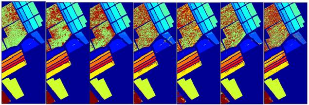
Figure 3 Mapping of classification results of various methods on the Salinas dataset

 

In order to observe the results, we draw a map of the classification results of each method.  In this experiment, 7 labeled sample points were randomly selected from each type of sample to form a training set.  All sample points are projected into low-dimensional space by learning the dimensionality reduction matrix through training set.  Classification and recognition are carried out in low dimensional space, and then the classification results are mapped with different colors.  As shown in Figure 3, there are 7 corresponding methods from left to right: (1)MDASSP(85.28%);  (2)DCNPE(84.36%);  (3)LADA(84.28%);  (4)DLPP(81.05%);  (5)KPCA(80.51%);  (6)SPP(80.46%);  (7)NPE(74.45%).  The corresponding classification accuracy is in parentheses.  Among them, the map of MDASSP method is the smoothest, because it has the least error sample points.  Especially in vineyard areas (the largest subdivision), there are fewer misfractions than other methods.  In addition, the classification accuracy of celery field and corn field is close to 1.  

 

4.    CONCLUSIONS AND RECOMMENDATIONS

This paper aims to solve the problem of "dimensional disaster" of hyperspectral image data.  Sparse representation and manifold learning are combined to reduce the dimension of hyperspectral data.  The two methods are combined to form a constrained optimization problem.  The effective projection matrix is obtained by optimizing the solution of the problem, and the projection data is classified and recognized.  Experimental results show that compared with other classification methods, the new method can improve the classification accuracy under small samples.  In the next step, we plan to combine a large number of unlabeled training sample points to build a semi-supervised learning algorithm.

 

 

 

REFERENCES

Azadeh Kianisarkaleh, Hassan Ghassemian (2016). Spatial-spectral Locality Preserving Projection for Hyperspectral Image Classification with Limited Training Samples, International Journal of Remote Sensing, 37(21):5045-5059. Retrieved   from https://doi.org/10.1080/01431161.2016.1226523

Deng S , Xu Y , He Y (2015), A hyperspectral Image Classification Framework and Its Application, Information Sciences, 299(1):379-393. Retrieved   from https://doi.org/10.1016/j.ins.2014.12.025

Dong S , Quan Y , Feng W (2021), A Pixel Cluster CNN and Spectral-Spatial Fusion Algorithm for Hyperspectral Image Classification With Small-Size Training Samples, IEEE Journal of Selected Topics in Applied Earth Observations and Remote Sensing, PP(99):1-1. Retrieved   from https://doi.org/10.1109/JSTARS.2021.3068864

Dongyang Wu, Li M A (2018), Multi-manifold LE Algorithm for Dimension Reduction and Classification of Multitemporal Hyperspectral Image, Remote Sensing for Land & Resources, 30(2): 80-86.

Efron B, Hastie T, Johnstone I (2004), Least Angle Regression, Ann Statist, 32(2):407-499. Retrieved   from https://doi.org/10.1214/009053604000000067

Feng Z, Yang S, Wang M (2019), Learning Dual Geometric Low-Rank Structure for Semisupervised Hyperspectral Image Classification, IEEE Transactions on Cybernetics, 10(1):1-13.

Fuding Xie, Cunkuan Lei, Fangfei Li (2019), Unsupervised Hyperspectral Feature Selection based on Fuzzy c-means and Grey Wolf Optimizer, International Journal of Remote Sensing, 40(9):3344-3367.Retrieved   from https://doi.org/10.1080/01431161.2018.1541366

Gao L , Yu H , Zhang B (2016), Locality-preserving Sparse Representation-based Classification in Hyperspectral Imagery, Journal of Applied Remote Sensing, 10(4): 42-54. Retrieved   from https://doi.org/10.1117/1.JRS.10.042004

Hairong Wang, Turgay Celik (2018). Sparse Representation-based Hyperspectral Image Classification, Signal Image & Video Processing, 12(5):1009-1017. Retrieved   from https://doi.org/10.1007/s11760-018-1249-1

Jayaprakash C , Damodaran B B , Viswanathan S (2020), Randomized Independent Component Analysis and Linear Discriminant Analysis Dimensionality Reduction Methods for Hyperspectral Image Classification, Journal of Applied Remote Sensing, 14(3). Retrieved   from https://doi.org/10.1117/1.JRS.14.036507

Lv M , Zhao X , Liu L (2017), Discriminant Collaborative Neighborhood Preserving Embedding for Hyperspectral Imagery, Journal of Applied Remote Sensing, , 11(4):1-17. Retrieved   from https://doi.org/10.1117/1.JRS.11.046004

Qi Wang, Zhaotie Meng, Xuelong Li. (2017) Locality Adaptive Discriminant Analysis for Spectral-Spatial Classification of Hyperspectral Images, IEEE Geoscience & Remote Sensing Letters, 14(11):2077-2081. Retrieved   from https://doi.org/10.1109/LGRS.2017.2751559

Qiao L , Chen S , Tan X (2010), Sparsity Preserving Projections with Applications to Face Recognition, Pattern Recognition, 43(1):331-341. Retrieved   from https://doi.org/10.1016/j.patcog.2009.05.005

Ren R, Bao W. (2019),Hyperspectral Image Classification Based on Belief Propagation with Multi-features and Small Sample Learning, Journal of the Indian Society of Remote Sensing, 47(5):1-10.Retrieved   from https://doi.org/10.1007/s12524-018-00934-y

Tabejamaat M , Mousavi A (2017), Manifold Sparsity Preserving Projection for Face and Palmprint Recognition, Multimedia Tools and Applications, 77(16):1-26. Retrieved   from https://doi.org/10.1007/s11042-017-4881-9

Uddin, Md. Palash, Mamun, Md. Al, Hossain, Md. Ali. (2019), Effective Feature Extraction Through Segmentation-based Folded-PCA for Hyperspectral Image Classification, International Journal of Remote Sensing, 40(18): 7190-7220. Retrieved   from https://doi.org/10.1080/01431161.2019.1601284

Wan Li, Liangpei Zhang, Lefei Zhang (2017), GPU Parallel Implementation of Isometric Mapping for Hyperspectral Classification, IEEE Geoscience & Remote Sensing Letters, 14(9): 1532 - 1536. Retrieved   from https://doi.org/10.1109/LGRS.2017.2720778

Wang A, Wang Y, Chen Y (2019). Hyperspectral Image Classification based on Convolutional Neural Network and Random Forest, Remote Sensing Letters, 10(11):1086-1094. Retrieved   from https://doi.org/10.1080/2150704X.2019.1649736

Xiangpo Wei, Xuchu Yu, Bing Liu (2019), Convolutional Neural Networks and Local Binary Patterns for Hyperspectral Image Classification , European Journal of Remote Sensing, 52(1):448-462.Retrieved   from https://doi.org/10.1080/22797254.2019.1634980

Yc A, Hl A, Liang Y A (2021), Hyperspectral Image Classification With Discriminative Manifold Broad Learning System, Neurocomputing.

Yongguang Zhai, Lifu Zhang, Nan Wang (2016), A Modified Locality-Preserving Projection Approach for Hyperspectral Image Classification, IEEE Geoscience & Remote Sensing Letters, 13(8):1059-1063. Retrieved   from https://doi.org/10.1109/LGRS.2016.2564993

Yuan Y, Wang C, Jiang Z (2021). Proxy-Based Deep Learning Framework for Spectral-Spatial Hyperspectral Image Classification: Efficient and Robust, IEEE Transactions on Geoscience and Remote Sensing, PP(99):1-15. Retrieved   from https://doi.org/10.1109/TGRS.2021.3054008