
|
|
|
|
BRAIN STROKE DETECTION USING TENSOR FACTORIZATION AND MACHINE LEARNING MODELSMosaad W. Hassan 1 1 Department of Mathematics (Computer Science), Faculty of Science, Tanta University, Egypt.2 Faculty of Computers and Information, Menofia University, Egypt. |
|
||
|
|
|||
|
Received 21 July 2021 Accepted 01 August2021 Published 15 August 2021 Corresponding Author Elham
Elfeky, elham.elfeky@science.tanta.edu.eg DOI 10.29121/ijetmr.v8.i8.2021.1006 Funding:
This
research received no specific grant from any funding agency in the public,
commercial, or not-for-profit sectors. Copyright:
© 2021
The Author(s). This is an open access article distributed under the terms of
the Creative Commons Attribution License, which permits unrestricted use, distribution,
and reproduction in any medium, provided the original author and source are
credited.
|
ABSTRACT |
|
|
|
Stroke is one
of the foremost common disorders among the elderly. Early detection of stroke
from Magnetic Resonance Imaging (MRI) is typically based on the
representation method of these images. Representing MRI slices in two
dimensional structures (matrices) implies ignoring the dependencies between
these slices. Additionally, to combine all features exist in these slices
requires more computations and time. However, this results in inexact
diagnosis. In this paper, we propose a new tensor-based approach for stroke
detection from MRI. The proposed methodology has two phases. In first phase,
each patient’s MRI are represented as a tensor. Tensor representations are
powerful because they capture the dependencies in high-dimensional data, MRI
of patient, which gives more reliable and accurate results. Also, tensor
factorization is used as a method for feature extraction and reduction, which
improves the performance and accuracy of classifiers. In second phase, these
extracted features are used to train support vector machine (SVM) and XGBoost classifiers to classify MRI images into normal
and abnormal. The proposed method is assessed with MRI dataset, and the
conducted experiments illustrate the efficiency of this approach. It achieves
classification accuracy of 98%. |
|
||
|
Keywords: Brain Stroke, Tensor Factorization, Classification, Machine Learning,
SVM 1. INTRODUTION The term “stroke” means
disturbances of the cerebral circulation producing central neurological
deficits of acute or sub-acute onset Greene, J., &
Bone, I. (2007). Brain stroke
cause severe weakening. This disease affects the vessels that outfit the
brain with blood due to rupture or clogging of the vessels Chawla, M., Sharma, S.,
Sivaswamy, J., & Kishore, L. T. (2009,
September), Kesavamurthy,
T., Rani, S., & Malmurugan, N. (2009). Supports
neurons in a damaged brain area that cannot carry out brain activities due to
lack of oxygen Rekik, I., Allassonnière, S., Carpenter, T. K., & Wardlaw, J. M.
(2012). The stroke
consequences lead to long-term weakness or death because the affected area of
brain does not function Tang, F. H., Ng, D.
K., & Chow, D. H. (2011). The stroke
consequences are unique to every individual, and recovery from a stroke
different for every person. Computed tomography (CT) scans and (MRI) are two
of the best diagnostic procedures for stroke patients. This because imaging
checks permit for a perfect outlook of the head, containing the blood vessels
and tissue. Radiologists can detect ischemic stroke damage better with MRI
scans than with CT scans, according to the American Academy of Neurology
reported in 2010 This technology can identify a range of brain and blood
vascular disorders, as well as visualize |
|
||


minute tissue variations that are difficult to see with other imaging modalities like a CT scanner.
In many circumstances, MRI can reveal tissue abnormalities that are too small to be identified by CT or are in parts of the brain where CT cannot. As a result, we used an MRI scan in our research. There are three types of strokes in the brain:
1) Hemorrhage Stroke.
2) Ischemic Stroke
3) Transient ischemic attack (a warning or “mini-stroke”).
Among this types, Ischemic Stroke accounts for 80% to 85% of stroke. The artery that deliveries oxygen-rich blood to brain becomes blocked during this type of stroke. A bright patch inside a brain scan image (MRI) with high contrast relative to its surroundings is typically visible in the bleeding region Chawla, M., Sharma, S., Sivaswamy, J., & Kishore, L. T. (2009, September). An ischemic (infarct) stroke appears as a dark (hypo dense) zone with low contrast in comparison to its surroundings Nagalkar, V., & Agrawal, S. (2012).
We deal with data having multiway structure in many real-world applications which is sadly commonly disregarded. In certain cases, irregularity may be undetectable using matrix-based spectral approaches. Besides, neglecting the multiway structure in data can cause some problems and lead to inaccurate results. To detect stroke from MRI, considering only a couple of biomarkers are not enough to give exact diagnosis.
The main contribution of this paper is to introduce an effective approach for detecting stroke that captures all relationships between different slices in MRI of individual patients.
Therefore, tensor is considered as a tool to represent the different slices in MRI of individual patients. Tensor representations are more powerful because they capture the relationships for high-dimensional data, MRI of patient, which gives more reliable and accurate results. Tensor factorization is applied to reduce features without affecting the relationships in the original tensor. This results in a core tensor, which is a shorthand for the original tensor. Also, it reflects all relationships that exist in the original tensor. Thus, the features of core tensor can be passed as inputs to the classifier.
The rest of the paper is organized as follows. Section 2 presents the related work to brain stroke diagnosis. Section 3 presents the preliminary definitions. Section 4 introduces the new proposed approach. Section 5 presents the experiment results and evaluation. Finally, section 6 presents conclusion and possible future work.
2. RELATEDWORK
In this section we identify the state of the art of automated brain stroke diagnosis. All existing methods for diagnosing stroke from MRI have been based principally on the matrix representation of MRI data.
In Gaidhani, B. R., Rajamenakshi, R. R., & Sonavane, S. (2019, September) Convolutional Neural Network (CNN) used to separate a normal tissue from an abnormal tissue. The method used in this research relies on three stages, pre-processing, classification using LeNet model, and segmentation using SegNet model. The deep learning models used for classification and segmentation require large memory, large data set, and lot of time to runs. In addition, this model produces inaccurate results as discussed in section5.3.
In Rajini, N. H., & Bhavani, R. (2013) segmentation approach used to separate a normal tissue from an abnormal tissue. The method in this paper is divided into four stages, pre-processing, tracking brain midline, feature extraction, and classification. For classification, k-nearest neighbors (KNN) and SVM are used. But it requires a large memory and results are inaccurate.
In Gupta, S., Mishra, A., & Menaka, R. (2014, May) image processing techniques are used to give an automated algorithm for brain stroke detection. The method used in this research relies on six phases: collected data in the form of MRI images, pre-processing data, tracing midline to obtain a symmetric image, image bifurcation, form the image quality matrix for analyze texture, and finally for classification they used neural network to separate normal and abnormal brain. The deep learning model used for classification require large memory, large data set, and more time to run.
Previous studies while representing the data did not take into consideration the relationships between different images of the same patient, which would have a strong influence on the accuracy of the diagnosis. To overcome these problems, we use, for each individual patient, a tensor structure to represent different his MRI’s slices. The representations of tensor are very helpful as they will capture relations between high-dimensional data, which makes diagnostics more accurate. This is shown in its results. We also focused on the importance of saving time by using an effective feature reduction way via Tucker decomposition. The target of this study to develop fast and reliable method which automatically diagnose brain stroke and delineate abnormal cases accurately.
3. PRELIMINARY DEFINITIONS
3.1. TENSOR
Definition1: A tensor is just a generalization of a vector (first order tensor), a matrix (second order tensor) to higher dimensions. An N-order tensor is defined as:
![]() (1)
(1)
Third-order tensor X has three types of fibers:
mode-1: column fibers denoted x_ (: jk)
mode-2: row fibers denoted x_(i:k)
mode-3: tube fibers denoted x_ (ij:)
Where colon (:) is used to indicate all elements of corresponding mode. Fibers are assumed to be column vectors. Fibers are the higher-order analogue of matrix columns and rows.
Third-order tensor X has three types of slices:
horizontal slices denoted X_(i∷)
lateral slices denoted X_ (: j:)
frontal slices denoted X_(∷k)
Slices are two-dimensional section of a tensor.
The order (or mode) of a tensor is the number of dimensions of data. The number of modes during a tensor is additionally referred to as the order of the tensor. Tensors, as natural generalizations of vectors and matrices, are becoming increasingly popular for representing multimodality data. A detail about tensors can be found in Kolda, T. G., & Bader, B. W. (2009), Bader, B. W., & Kolda, T. G. (2007).
Definition2: The n-mode product (denoted by ×n)
of a tensor ![]() with a matrix
with a matrix ![]() is a tensor
is a tensor![]() , denoted as:
, denoted as:
![]() (2)
(2)
Where each entry of Y is defined as the sum of products of corresponding entries in X and U Lu, H., Plataniotis, K. N., & Venetsanopoulos, A. (2013).
Definition3: Let ![]() ,
the
,
the ![]() of
of ![]() ,
denoted
,
denoted ![]() is the dimension of the vector space spanned
by the mode-n fibers.
is the dimension of the vector space spanned
by the mode-n fibers.
![]() (3)
(3)
Where ![]() are the unfolding on mode-k.
are the unfolding on mode-k.
If ![]() then we can say that X is a
then we can say that X is a ![]() tensor. The N-tupple
tensor. The N-tupple ![]() is known as the multi-linear rank of tensor
is known as the multi-linear rank of tensor ![]() Lu, H., Plataniotis, K. N.,
& Venetsanopoulos, A. (2013).
Lu, H., Plataniotis, K. N.,
& Venetsanopoulos, A. (2013).
Definition4: (Vectorization: tensor to vector
transformation). The vectorization of a tensor is a linear transformation that
converts the tensor ![]() into
a column vector
into
a column vector ![]() Lu, H., Plataniotis, K. N.,
& Venetsanopoulos, A. (2013), denoted as:
Lu, H., Plataniotis, K. N.,
& Venetsanopoulos, A. (2013), denoted as:
![]() (4)
(4)
3.2. TENSOR DECOMPOSITION (FACTORIZATION)
Tensor factorization is used to find connections and correlations between various modes of high dimensional data. Tensor factorization is a generalization of matrix factorization algorithms such as singular value decomposition (SVD) or principal component analysis (PCA), and it makes use of information from the multiway structure that is lost when modes are collapsed Kolda, T. G., & Bader, B. W. (2009), Mørup, M. (2011),Lu, H., Plataniotis, K. N., & Venetsanopoulos, A. N. (2011) Wang, D., & Kong, S. (2012). Among many types of tensor factorization methods, Tucker model is the most used one Bader, B. W., & Kolda, T. G. (2007), Tucker, L. R. (1966). Tucker decomposition can be seen as a form of higher-order principal component analysis Tucker, L. R. (1966), Tucker, L. R. (1964), Tucker, L. R. (1963), is also known as higher-order singular value decomposition (SVD) De Lathauwer, L., De Moor, B., & Vandewalle, J. (2000), and N-mode principal component analysis Kroonenberg, P. M., & De Leeuw, J. (1980). It decomposes the N-order data tensor X into N factor matrices multiplied by a core tensor G. Factor matrices specify groups in each mode. Core tensor specifies the levels of interaction between the groups from different modes.
In 4-orser tensor, the original tensor ![]() can be expressed as a series of 4-mode
products between the core tensor G and the factor matrices
can be expressed as a series of 4-mode
products between the core tensor G and the factor matrices ![]() and
and ![]() .
.
![]() (5)
(5)
![]() (6)
(6)
Where![]() ,
,![]() ,
,
![]() ,
and
,
and ![]() are the factor matrices (Which are usually
orthogonal) and can be thought of as the principal components in each mode. The
tensor
are the factor matrices (Which are usually
orthogonal) and can be thought of as the principal components in each mode. The
tensor ![]() is called the core tensor and its entries show
the extend of interaction among the various components. From equation (5) the
core tensor
is called the core tensor and its entries show
the extend of interaction among the various components. From equation (5) the
core tensor ![]() can be obtained as follows:
can be obtained as follows:
![]() (7)
(7)
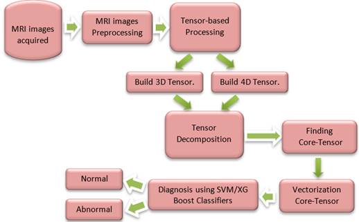
4. PROPOSED METHODOLOGY
Our approach is essentially consisting of three steps:
Step 1: MRI pre-processing: this step is required to improve the quality of MRI image and provide good details before feature extraction performed by tensor. In practical, MRI of patient consists of three sections of slices (2D images): horizontal, lateral, and frontal slices. Each of these sections contains different number of slices. Here, the size of all slices is adapted to be 256 × 256.
Step 2: Tensor-based processing: in this step we do two tasks:
First task: Building a tensor. In this paper we apply our approach with 3-order (3D) tensors and 4-order (4D) tensors. 3D tensor (256 × 256 × 600) is created by considering the spatial (voxel) dimensions as two modes with size 256 × 256, and the third mode corresponding to the total number of slices for each patient (600 slices). 4D tensor (256 × 256 × 189 × 3) is created by considering the spatial (voxel) dimensions as two modes with size 256 × 256, the third mode corresponding to the smallest number of slices for each aspect (189 slices), and the fourth way corresponding to the number of aspects (three aspects). Aspects here refers to orientations: horizontal, lateral, and frontal. When all aspects do not have the same number of MRI slices, we consider the smallest number and choose the same number randomly from the other two aspects.
Second task: Feature reduction: Tucker decomposition is used with 3D and 4D tensors with multi-linear ranks (8 × 7 × 25) and (8 × 7 × 5 × 3) respectively. Then the core tensors in two cases are obtained and transformed into vectors. At the end of this step, each patient will be presented as a vector. This vector represents the extracted features that are most useful in training the classifiers.
Step 3: Classification: The vectors group result
in previous step became the gateway to machine learning models. These vectors
are passed as input patterns to two classifiers SVM Steinwart, I., & Christmann,
A. (2008), Kavitha, M., Lavanya, G., & Janani, J. (2018) and XG Boost Long, H. E. (2020). The MRI images of
each patient are classified into normal (0) and abnormal (1). Finally, the
accuracy with each classifier in the two cases are computed. The proposed
approach is shown in Figure 1The complete proposed
algorithm is summarized in Algorithm 1
|
Algorithm 1: The algorithm for new proposed system
is illustrated as follows: |
|
Input: set of normal and abnormal MRI images for brain stroke patients. |
|
Output: classification of MRI images into two classes, normal and
abnormal. |
|
1-
Define |
|
2-
for each patient P do |
|
3-
Perform
image pre-processing, as in step1. |
|
4-
Construct
N-order tensor |
|
5-
Find
core tensor |
|
6-
Vectorize
core tensor |
|
7-
Add each
vector to the list |
|
8-
Label
normal patient images as 0 and abnormal patient images as 1; |
|
9-
end for |
|
10-
Run SVM
and XGBoost on |
|
|
|
Figure 1: Proposed Methodology |
5. EXPERIMENTS AND ANALYSIS
5.1. DATASET DESCRIPTION
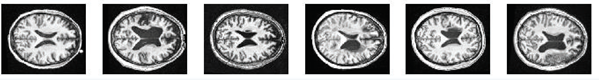
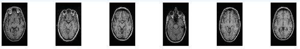
Our approach is evaluated on MRI dataset for stroke detection tasks that is acquired from two places. One is collected from Tanta University hospitals. We encountered many difficulties and challenges during the data collection process. The obtained MRI data was in DCM format and contain 100 MRI images (39 Normal and 61 abnormal). The other is obtained from ATLAS (Anatomical Tracings of Lesions after Stroke), website mainly for neuroimaging studies Liew, Sook-Lei 2018. This dataset contains 200 T1-weighted MRI images (90 normal and 110 Abnormal). After performing pre-processing, 300 MRI scans are selected for the experiments (129 normal and 171 abnormal). This data is in Nifti format. All MRI images are adapted in JPG format and each one is normalized to a 256 ´ 256 gray images. For instance, Figure 2 and Figure 3 show abnormal and normal patient images.
|
|
|
Figure 2: Abnormal Axial Images |
|
|
|
Figure 3: Normal Axial Images |
5.2. EXPERIMENTAL RESULTS
The python is used to implement the proposed approach. We run the implementation on Processor: Intel(R) Core (TM) i7-8550U CPU @ 1.80GHz 1.99 GHz, and RAM: 16 GB. Our approach is evaluated on candidate dataset which contain 300 MRI images (129 normal and 171 abnormal). The dataset is divided into two parts 70% data for training and 30% data for testing. These dataset of 300 MRI images are adapted to construct 3D and 4D tensors of features. Then Tucker decomposition is performed to extract core tensor which contains the reduced features. SVM and XG Boost classifiers are used for classifying the MRI images into normal and abnormal. To optimize the parameters of the classifiers, we use grid search algorithm to find the best combination of hyper-parameters for a given model (e.g., an SVM) and test dataset. Grid Search is a technique for determining the best hyper-parameters and thereby improving accuracy.
In the context of conducted experiments, we used multilinear perceptron (MLP) Atienza, R. (2020) neural network model. Two paths are applied in this experiment based on the dimension of core tensor which represents the patient. In the first path, the 4-dimensional core tensor is used as input to MLP model with shape (8, 7, 5, 3). The MLP model consists of six fully connected layers with 840, 420, 210, 105, 55 and 30 units, respectively. Then, each of these layers are followed by Rectified Linear unit (ReLU) activation funation and dropout layer [29]. In the second path, the 3D core tensor is utilized as input to MLP model with shape (8, 7, 25). Then in MLP model, seven fully connected layers are used with 1400, 700, 350, 125, 60, 30 and 15 units, respectively. Each of these fully connected layers are followed by ReLU function and dropout layer.
We evaluate our results of proposed method using accuracy. One statistic for evaluating classification is accuracy, which is the percentage of correct predictions made by our model. The following is the formal definition of accuracy:
![]()
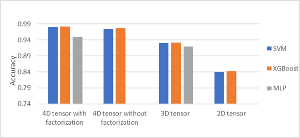
According to Algorithm 1, Table 1presents experimental results of 4-order tensor with factorization, 4-order tensor without factorization, 3-order tensor, and 2-order tensor (matrix). We note that the best result obtained with 4D tensor of size (256 × 256 × 189 × 3) with factorization via multi-liner ranks (8, 7, 5, 3). The core tensor is vectorized into vector of size (840 × 1). These features are passed as input to the classifiers SVM, XGBoost. In addition, as shown from table1 the proposed method based on SVM and XGBoost achieves higher performance than MLP method. Further, Figure 4 shows the accuracy obtained of three classifiers; SVM, XGBoost, and MLP.
|
Table 1: The Accuracy Result for The Proposed
Method |
||||||||
|
|
4D tensor with factorization
(256´256´189´3) |
4D tensor without
factorization (256´256´189´3) |
3D tensor (256´256´567) |
2D tensor (65536´567) |
||||
|
|
Accuracy |
No. of features |
Accuracy |
No. of features |
Accuracy |
No. of features |
Accuracy |
No. of features |
|
SVM |
0.98 |
840 |
0.975 |
37158912 |
0.93 |
1400 |
0.84 |
12500 |
|
XG Boost |
0.982 |
840 |
0.977 |
37158912 |
0.932 |
1400 |
0.842 |
12500 |
|
MLP |
0.95 |
840 |
- |
- |
0.92 |
1400 |
- |
- |
|
|
|
Figure 4: Accuracy for brain stroke
classification using SVM, XGBoost and MLP |
5.3. COMPARISON WITH OTHER METHODS
We compare our approach with the CNN method in Gaidhani, B. R., Rajamenakshi, R. R., & Sonavane, S. (2019, September) relied on using convolutional neural network (LeNet model) for classification. The CNN method neglected the important connection between all slices of single patient. This forced to ask the
radiologist for helping in carefully identifying the affected area. This may cause the consumption of time and effort. Also, the precision of diagnosis is relatively infected by neglecting important dependences between slices. This is completely inconsistent with the concept of precision medicine, which aims to take everything related to the patient into consideration for accurately diagnose. Another main problem is arising in using the slices of patient separately. This leads to more combinations in trying to take all patient images into consideration. Sometimes, these combinations need several computing devices with special specifications. This increases the cost in addition to the time spent during implementation.
To overcome above defects, tensor factorization has emerged as a promising solution for these challenges. It can be applied at the lowest costs, least time and with the best results. From the evaluation results that we obtained by randomly selecting the data set several times, it turns out that the performance is better when using tensor factorization method as shown in Figure 5. Moreover, several performance metrics results are used for the new method is more accurate than the CNN method as shown in Table 2.
|
|
|
Figure 5:
Experimental results: accuracy for randomly selecting data set using Tensor
and LeNet models |
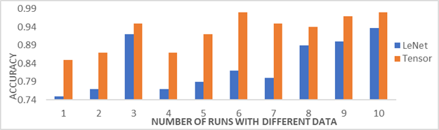
From the evaluation results shown in Table 2 the rates of metrics for our method are better than CNN method that use LeNet model for classification.
|
Table 2: Comparison Between Cnn and Our Method Using Accuracy, Precision, Recall, And
F_Measure Metrics to Evaluate Performance |
||||
|
|
Accuracy
of average of 10 runs |
Precision
of average of 10 runs |
Recall
of average of 10 runs |
F_measure of average of 10 runs |
|
Proposed
tensor-based model |
98% |
97.3 |
99.2 |
98.6 |
|
LeNet
model |
93.8% |
94.1 |
94.3 |
94.2 |
6. CONCLUSION AND FUTUREWORK
In this work, we have advanced a tensor-based technique to optimize the process of stroke diagnosis from MRI images. The tensor-based approach has several Properties: 1) it captures all dependencies between MRI slices for each individual patient via tensor (higher-order) representation; 2) it reduces the number of input features in the learning process, efficiently, via tensor decomposition; 3) it types better use of all information presented in MRI images; 4) it converges in less time than CNN; and 5) its accuracy is better than previous methods. The experimental results shows that tensor-based approach outdoes CNN in terms of classification accuracy and convergence. In future, we aim at expanding the approach to classify the abnormal MRI images into more classes. That is, the model can handle large sets of MRI images and identify one or more brain disease with high precision.
REFERENCES
Atienza, R. (2020). Advanced Deep Learning with TensorFlow 2 and Keras: Apply DL, GANs, VAEs, deep RL, unsupervised learning, object detection and segmentation, and more. Packt Publishing Ltd.
Bader, B. W., & Kolda, T. G. (2007). Tensor decompositions and their application (No. SAND2007-4390C). Sandia National Lab. (SNL-NM), Albuquerque, NM (United States); Sandia National Laboratories, Livermore, CA. Retrieved from https://www.osti.gov/servlets/purl/1147546
Chawla, M., Sharma, S., Sivaswamy, J., & Kishore, L. T. (2009, September). A method for automatic detection and classification of stroke from brain CT images. In 2009 Annual international conference of the IEEE engineering in medicine and biology society (pp. 3581-3584). IEEE. DOI : 10.1109/IEMBS.2009.5335289
De Lathauwer, L., De Moor, B., & Vandewalle, J. (2000). A multilinear singular value decomposition. SIAM journal on Matrix Analysis and Applications, 21(4), 1253-1278. Retrieved from https://doi.org/10.1137/S0895479896305696
Gaidhani, B. R., Rajamenakshi, R. R., & Sonavane, S. (2019, September). Brain Stroke Detection Using Convolutional Neural Network and Deep Learning Models. In 2019 2nd International Conference on Intelligent Communication and Computational Techniques (ICCT) (pp. 242-249). IEEE. DOI: 10.1109/ICCT46177.2019.8969052
Greene, J., & Bone, I. (2007). Understanding neurology: A problem-oriented approach. CRC Press.
Gupta, S., Mishra, A., & Menaka, R. (2014, May). Ischemic Stroke detection using Image processing and ANN. In 2014 IEEE International Conference on Advanced Communications, Control and Computing Technologies (pp. 1416-1420). IEEE. DOI : 10.1109/ICACCCT.2014.7019334
Kavitha, M., Lavanya, G., & Janani, J. (2018). Enhanced SVM classifier for breast cancer diagnosis. International Journal of Engineering Technologies and Management Research, 5(3), 67-74. Retrieved from https://doi.org/10.29121/ijetmr.v5.i3.2018.178
Kesavamurthy, T., Rani, S., & Malmurugan, N. (2009). EARLY DIAGNOSIS OF ACUTE BRAIN INFARCT USING GABOR FILTER TECHNIQUE FOR COMPUTED TOMOGRAPHY IMAGES (< Special Issue> Biosensors: Data Acquisition, Processing and Control). International Journal of Biomedical Soft Computing and Human Sciences: the official journal of the Biomedical Fuzzy Systems Association, 14(2), 11-16. Retrieved from https://doi.org/10.24466/ijbschs.14.2_11
Kolda, T. G., & Bader, B. W. (2009). Tensor decompositions and applications. SIAM review, 51(3), 455-500. Retrieved from https://doi.org/10.1137/07070111X
Kroonenberg, P. M., & De Leeuw, J. (1980). Principal component analysis of three-mode data by means of alternating least squares algorithms. Psychometrika, 45(1), 69-97. Retrieved from https://doi.org/10.1007/BF02293599
Lansberg, M. G., Albers, G. W., Beaulieu, C., & Marks, M. P. (2000). Comparison of diffusion-weighted MRI and CT in acute stroke. Neurology, 54(8), 1557-1561. Retrieved from https://doi.org/10.1212/WNL.54.8.1557
Long, H. E. (2020). Depth understanding XGBoost: Efficient and advanced machine learning algorithms (Chinese Edition). Machinery Industry Press.
Liew, Sook-Lei 2018. The Anatomical Tracings of Lesions after Stroke (ATLAS) Dataset - Release 1.2, Inter-university Consortium for Political and Social Research [distributor], 2018-11-27 Retrieved from. https://doi.org/10.3886/ICPSR36684.v3
Lu, H., Plataniotis, K. N., & Venetsanopoulos, A. (2013). Multilinear subspace learning: dimensionality reduction of multidimensional data. CRC press.
Lu, H., Plataniotis, K. N., & Venetsanopoulos, A. N. (2011). A survey of multilinear subspace learning for tensor data. Pattern Recognition, 44(7), 1540-1551. Retrieved from https://doi.org/10.1016/j.patcog.2011.01.004
Mørup, M. (2011). Applications of tensor (multiway array) factorizations and decompositions in data mining. Wiley Interdisciplinary Reviews: Data Mining and Knowledge Discovery, 1(1), 24-40. Retrieved from https://doi.org/10.1002/widm.1
Mørup, M. (2011). Applications of tensor (multiway array) factorizations and decompositions in data mining. Wiley Interdisciplinary Reviews: Data Mining and Knowledge Discovery, 1(1), 24-40. Retrieved from https://doi.org/10.1002/widm.1 DOI : 10.1002/widm.1
Nagalkar, V., & Agrawal, S. (2012). Ischemic stroke detection using digital image processing by fuzzy methods. International Journal of Latest Research in Science and Technology, 1(4), 345-347.
Rekik, I., Allassonnière, S., Carpenter, T. K., & Wardlaw, J. M. (2012). Medical image analysis methods in MR/CT-imaged acute-subacute ischemic stroke lesion: Segmentation, prediction and insights into dynamic evolution simulation models. A critical appraisal. NeuroImage: Clinical, 1(1), 164-178. Retrieved from https://doi.org/10.1016/j.nicl.2012.10.003
Smilde, A., Bro, R., & Geladi, P. (2005). Multi-way analysis: applications in the chemical sciences. John Wiley & Sons.
Steinwart, I., & Christmann, A. (2008). Support vector machines. Springer Science & Business Media.
Tang, F. H., Ng, D. K., & Chow, D. H. (2011). An image feature approach for computer-aided detection of ischemic stroke. Computers in biology and medicine, 41(7), 529-536. Retrieved from https://doi.org/10.1016/j.compbiomed.2011.05.001
Tucker, L. R. (1963). Implications of factor analysis of three-way matrices for measurement of change. Problems in measuring change, 15(122-137), 3.
Tucker, L. R. (1964). The extension of factor analysis to three-dimensional matrices. Contributions to mathematical psychology, 110119.
Tucker, L. R. (1966). Some mathematical notes on three-mode factor analysis. Psychometrika, 31(3), 279-311. Retrieved from https://doi.org/10.1007/BF02289464
Wang, D., & Kong, S. (2012). Feature selection from high-order tensorial data via sparse decomposition. Pattern Recognition Letters, 33(13), 1695-1702. Retrieved from https://doi.org/10.1016/j.patrec.2012.06.010
Rajini, N. H., & Bhavani, R. (2013). Computer aided detection of ischemic stroke using segmentation and texture features. Measurement, 46(6), 1865-1874. Retrieved from https://doi.org/10.1016/j.measurement.2013.01.010
|
|
 This work is licensed under a: Creative Commons Attribution 4.0 International License
© IJETMR 2014-2021. All Rights Reserved.