
|
|
|
|
Original Article
SUSTAINABLE INVENTORY MODEL FOR OPTIMIZING GREENHOUSE INVENTORY MANAGEMENT THROUGH SUSTAINABLE PRACTICES
|
Archit Jain 1* 1 Scholar, Institute, Digamber Jain College, Baraut, UttarPradesh,
India 2 Professor & Supervisor, Institute, Digamber Jain College, Baraut, UttarPradesh, India |
|
|
|
ABSTRACT |
||
|
The major source of the variance in the environmental system is the dramatic increase in carbon emission (CO2). Deterioration on the massive scale is compelled in the green house companies due to the fact that green product is life cycle very limited (summer). The modern companies (green companies especially) are striving to simplify their current inventories processes so as to carry out the maximum profitability in terms of the environmental issues. To gain the economic and ecological benefits, they must make a sustainable system of inventory. The second similarity to the modern inventory system is the inflation factor that has steadily risen throughout the years during the pandemic of COVID-19 to most of the items. Due to the topicality of these concerns, the contemporary study focuses on the notion of green technology investment to prevent not only the carbon release produced by the use of the transport system but also the application of preservation technology to control the disintegrating character of the latter under the impact of inflation. The existing model was considered to be an economic order quantity model having a scheme of advance payment, the variable holding cost, and the demand rate based on the size of the amount on hand. A number of sub cases have been performed through the use of numerical examples to test the validity of the proposed model. The sensitivity analysis depicts the observation of the positive effects of controllable deterioration and emission of carbon. The results revealed that the system cost cuts by 5.96 percent as a result of putting funds in the green technology and preservation technology. Keywords: Sustainability, Inventory, Green
technology, Preservation, Deterioration, Inflation, Carbonemission,
Optimization |
||


INTRODUCTION
The major problems, the whole world is facing, are
environmental difficulties. The main cause which is responsible to harm the
environment is continuously increasing carbon emission from industries and
transporting system Mashud
et al. (2021),Pando et al. (2013),Sarkar et al. (2014). Production
companies release Carbon Dioxide (CO2), which is also called
greenhouse gas harms the earth. The main loss due to carbon emission is climate
changing, most popularly global warming. Most of the carbon emission comes from
transportation and inventory holding system Jawla
and Singh (2016), Lashgari
et al. (2016), Shi et al. (2020). The Governments of
many countries are trying to deduct the environmental loss due to greenhouse
carbon emissions which are produced through transport Chandra
et al. (2020),Chang et al. (2019), which devotes to a
quarter of the entire carbon emissions Taleizadeh et
al. (2013),Teng et al. (2016). They are motivating
towards the latest inventions of green technologies (GT) as green technologies
are the only solution to control carbon emissions and developed a sustainable
inventory model. Yu and Hui (2008) developed a
sustainable inventory model which provides inventive methods to control the
loss due to pollutant emission Yu and Hui (2008). Lou et al., (2015)
discussed an inventory system that reduced carbon emission with the help of
green technology Lou et al. (2015).
Deterioration is another major task to handle in the
current inventory system. Most of the agricultural items have to go through
deterioration. In this context, preservation technologies take place to control
the deterioration. Plants and flowers retailer always invest in preservation
technology (PT) as they have a short life cycle so that they need some
facilities to maintain their quality for a certain time. Many researchers
considered the PT investment in their models Zauberman et
al. (1991), Chen et al. (2020), Datta et
al. (2020), Khanna
et al. (2020), Zulu et al. (2020). To establish a
sustainable inventory system, investment in both preservation and green
techniques is required Gaur et al. (2020). It will turn down
the retailer’s loss due to deterioration as well as will provide a healthy
environment. Mishra
et al. (2020) developed a model by
considering a joint investment of preservation technology and green technology
for a greenhouse flower company Mishra
et al. (2020). Mashud
et al. (2021) projected a
sustainable inventory model. Their proposed green technology investment is
beneficial to curb carbon emissions produced from transporting system Mashud
et al. (2021) Wu et al. (2018).
PROBLEM DEFINITION
To fill this gap, the proposed study developed a SEOQ
model which invests in both PT and GT simultaneously. The minimum cost is
obtained and tried to reduce the carbon emission coming from the vehicle Chen et al. (2019). This research is
aimed to develop a model for a retailer that can minimize its cost with less
environmental loss Pervin
et al. (2020). Fruits and
vegetables are the major products, considered in this research as they are much
vulnerable Kumar et
al. (2020). This study also
considered the payment problems occurring in COVID-19, a supplier offers an
advance payment policy to its retailers that retailers can pay the full amount
in multiple installments as most of the people could
not hold a huge amount of money in this pandemic to pay full payment in a
single installment Mishra
et al. (2020). In this pandemic,
inflation is one such factor that cannot be ignored Banerjee
et al. (2018), Li et al. (2018). Most of the
products especially food items faced high inflation during this time. This
study would be helpful for retailers to minimize their cost taking inflation
into the account Datta
(2017) Tripathi
et al. (2018), Das et al. (2021). Also, it is not
mandatory that inflation always increases the total cost, it can be optimized
by investing in preservation and green technology. Table 1 shows a quick
comparison of available research and propose research Shah et al. (2020), Giri et al. (2017).
|
Table 1 |
|
Table
1 Sustainable Greenhouse Inventory Model |
|||||||||
|
Authors |
Stock-dependent demand |
Price dependent demand |
Deterioration |
Carbon emission |
PT investment |
Advance payment |
Time varying holding cost |
Inflation |
GT investment |
|
Shah et al. (2014) |
✓ |
✓ |
✓ |
✓ |
|||||
|
Jawla et al. (2016) |
✓ |
✓ |
✓ |
✓ |
|||||
|
Tripathi et al. (2018) |
✓ |
✓ |
|||||||
|
Datta et al. (2019) |
✓ |
✓ |
✓ |
✓ |
|||||
|
Shi et al. (2019) |
✓ |
||||||||
|
Gaur et al. (2020) |
✓ |
✓ |
✓ |
||||||
|
Kumar et al. (2020) |
✓ |
✓ |
✓ |
✓ |
|||||
|
Shah et al. (2020) |
✓ |
✓ |
✓ |
||||||
|
Pervin et al. (2020) |
✓ |
✓ |
✓ |
✓ |
|||||
|
Das et al. (2021) |
✓ |
✓ |
✓ |
||||||
|
Present Paper |
✓ |
✓ |
✓ |
✓ |
✓ |
✓ |
✓ |
✓ |
✓ |
NOTATIONS AND HYPOTHESIS
The present inventory system consists of some specific
notations and the assumptions made to develop the model.
Notations
The notations are divided into two parts: decision
variables and constant parameters, as follows:
Decision Variables
![]() :
Investment in PT / unit time
:
Investment in PT / unit time
![]() : Length
of system cycle
: Length
of system cycle
Constant Parameters
· ![]() : Stock
level at any time
: Stock
level at any time
· ![]() : Lead
time
: Lead
time
· ![]() : Maximum
inventory
: Maximum
inventory
· ![]() : Holding
cost / unit / unit time at any time
: Holding
cost / unit / unit time at any time ![]()
·
![]() :
Deterioration cost / unit
:
Deterioration cost / unit
· ![]() :
Inflation rate
:
Inflation rate
· ![]() : Selling
price rate
: Selling
price rate
·
![]() : Ordering
cost / order
: Ordering
cost / order
·
![]() :
Purchasing cost / order
:
Purchasing cost / order
·
![]() :
Deterioration rate without investment in PT
:
Deterioration rate without investment in PT
· ![]() :
Deterioration rate with investment in PT
:
Deterioration rate with investment in PT
· ![]() : Number
of trips
: Number
of trips
·
![]() : Fixed
transportation cost
: Fixed
transportation cost
·
![]() : Fuel
amount vehicle consumes when empty
: Fuel
amount vehicle consumes when empty
·
![]() : Extra
vehicle fuel consumption/ton payload
: Extra
vehicle fuel consumption/ton payload
· ![]() : Amount
to be paid before delivery
: Amount
to be paid before delivery
·
![]() : The same
amount variable transportation cost to fuel price
: The same
amount variable transportation cost to fuel price
·
![]() : Vehicle
generates carbon emission cost
: Vehicle
generates carbon emission cost
·
![]() :
Additional carbon emission cost
:
Additional carbon emission cost
·
![]() : Distance
travelled from supplier to retailer and then to consumer
: Distance
travelled from supplier to retailer and then to consumer
· ![]() : Maximum
reduced amount of carbon emission when GT invested,
: Maximum
reduced amount of carbon emission when GT invested, ![]()
· ![]() : The
efficiency of GT in declining emission,
: The
efficiency of GT in declining emission, ![]()
· ![]() : Discrete
quantity of investment in GT ($/year)
: Discrete
quantity of investment in GT ($/year)
Hypothesis
The following hypotheses have been inserted into the
development of the proposed model:
The holding cost is taken as a linear function of
time, i.e.
![]()
1)
The model considers the inflation effect with rate ![]() , where
, where ![]() .
.
2)
The demand rate is correlated to the selling price and
stock level, i.e.
![]()
1)
Instantaneous deterioration arises for all items at a
constant rate ![]() .
.
2)
The model invests in preservation technologies to
control deterioration. For preservation technology investment, the following
function is used:
![]()
which satisfies the conditions:
![]()
where ![]() is the
sensitivity parameter of investment,
is the
sensitivity parameter of investment, ![]() .
.
1)
In the case of advance payment, the leading time is
constant. Otherwise, the lead time assumed in the present model is close to
zero for the case of no advance payment.
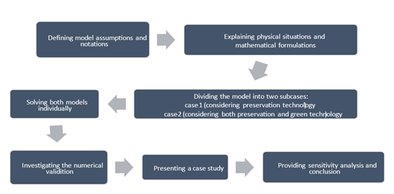
MATHEMATICAL FORMULATIONS
This model has divided into two different parts where
the first part involves product deterioration reduction using the preservation
technologies while the second part involves product deterioration reduction
with green technologies to reduce the joint loss due to deterioration and
carbon emission Hsieh
and Dye (2017). For the reader’s
convenience to understand the adopted steps, the research methodology used in
the development of this model has given in Fig.7.1. A detailed explanation of
considered situations and corresponding models is given below. Balaman and
Selim (2016)
Case 1 (considering preservation technology)
An economic order quantity (EOQ) model is made in the
consideration of the hypothesis mentioned before. In the present time, the
business market is so much affected by COVID-19 in the reference of payments Singh et
al. (2016),Lou et al. (2015). Small retailers are
facing so many problems in this scenario as generall,
they hold a low amount of their capital. They need to pay a huge amount to the
supplier which is quite not possible in the time of COVID environment. The
other major problem the retailer is facing at present is inflation Yang et al. (2015). As inflation is
increasing for most of the products, it became hard to manage to pay the full
amount in a single installment Dye and Hsieh (2013). Keeping all this in
the mind, the supplier proposes a scheme of advance payment for the retailer to
reimburse for a part of the complete amount at the time of delivery of the item
Dye and Hsieh (2013). In the proposed
study, A retailer buys a Q unit of
items from the supplier. At the time of delivery, the supplier transports all
the items to the retailer after getting the remaining amount of payment.
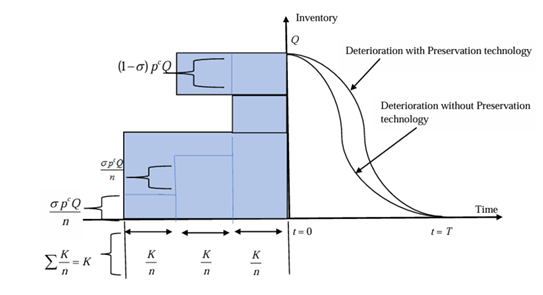
In Fig. 2., the physical situation of this inventory
system is shown. The retailer pays the product’s amount in several installments (n)
with the processing time (K). The
largest shaded part shows the total number of divisions of payment that have to
be paid before giving the items, whereas the next-largest shaded part
represents the leftover (1− ![]() ) percentage of the total amount. This amount was later
settled by the retailer on delivery of the items. Having the entire stock, the
retailer seeks to manage the consumer requirement. Unwillingly, deterioration
started at the initial stage (t = 0)
for all the items. To control the product’s deterioration, the retailer
invested in preservation technology. On account of consumer demand and
instantaneous deterioration, the stock level turns out to be zero at t = T.
) percentage of the total amount. This amount was later
settled by the retailer on delivery of the items. Having the entire stock, the
retailer seeks to manage the consumer requirement. Unwillingly, deterioration
started at the initial stage (t = 0)
for all the items. To control the product’s deterioration, the retailer
invested in preservation technology. On account of consumer demand and
instantaneous deterioration, the stock level turns out to be zero at t = T.
|
Figure 1
|
|
Figure 1 Research Methodology |
|
Figure 2 |
|
|
|
Figure 2 Graphical Inventory System |
The associated differential equation of the stock
level is taken as follows:
![]()
with initial boundary situation:
![]()
The solution of Eq. (1) using Eq. (2) is given by:
![]()
And so that the initial stock (at ![]() ) level is
given by:
) level is
given by:
![]()
Cost
Components
The associated cost functions are as follows:
a) Ordering cost per cycle:
![]()
b) The retailer tries to manage the deterioration in
products with the help of required preservation technology (PT) which consumes
the investment cost. The investment cost is given by:
![]()
c) Every retailer needs to hold the inventories until
they are traded. Thus, the variable holding cost per cycle is calculated as:
![]()
d) Purchase cost is the amount that is given to the
supplier by the retailer for his desired stock. If ![]() is the
overall stock (assumed earlier), then the total purchase cost (PC) per cycle is
given by:
is the
overall stock (assumed earlier), then the total purchase cost (PC) per cycle is
given by:
![]()
e) Retailers invested in preservation technology to
control deterioration which preserves the inventory but for a specific time.
So, the deterioration cost per cycle is stated by:
![]()
f) In this inventory system, stock level ![]() is
delivered by the supplier after getting the full amount of payment and then
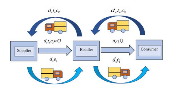
transported to the consumer from the retailer by paying the shipping cost. In Figure 3, the existing
transportation situation is shown. The supplier transports all the stock to the
retailer by truck Wahab et
al. (2011). The distance adds
up for the reverse process, so distance
is
delivered by the supplier after getting the full amount of payment and then
transported to the consumer from the retailer by paying the shipping cost. In Figure 3, the existing
transportation situation is shown. The supplier transports all the stock to the
retailer by truck Wahab et
al. (2011). The distance adds
up for the reverse process, so distance ![]() is added.
The truck generates carbon emission which is emergent on the purchased stock of
the vehicle payload and the extra carbon emission is also added after the
supplier transports stock to the retailer Hsieh
and Dye (2010). The total vehicle
fuel consumption is multiplied into the variable transportation cost. Hence,
the total transportation cost per cycle is given by:
is added.
The truck generates carbon emission which is emergent on the purchased stock of
the vehicle payload and the extra carbon emission is also added after the
supplier transports stock to the retailer Hsieh
and Dye (2010). The total vehicle
fuel consumption is multiplied into the variable transportation cost. Hence,
the total transportation cost per cycle is given by:
![]()
g) Before the time of delivery, the cyclic
capital cost for the retailer is (from Figure 2, referenced by Wu et al. (2018)):
![]()
(See Appendix A for detailed calculation)
Hence, the total cost can be calculated as:
![]()
The main aim of the present paper is to optimize ![]() and
and ![]() so that
so that ![]() is
minimized. The necessary conditions for the optimization of
is
minimized. The necessary conditions for the optimization of ![]() and
and ![]() are
followed by:
are
followed by:
![]()
and
![]()
The sufficient condition for the optimization of ![]() and
and ![]() is
followed by:
is
followed by:
![]()
The solutions of Eqs. The
spot (12) and (13) give graphs of the cycle length T and the investment
parameter T. This is due to the fact that all the mandatory derivatives are
computed in Appendix B. When these numbers are applied in the equation one will
be able to end up with most optimal inventory level. (4) [30]. The total cost
activity may also be mathematically presented as an equation below (15). This
is the cause why the overall cost monofunction TC' (τ,T) is:
![]()
![]()
![]()
![]()
|
Figure 3
|
|
Figure 3 Transportation
System |
Case-2 (Considering Both Preservation and Green Technology)
At present, the environment is facing major problems
due to carbon emissions. All fuel vehicles are the main cause of carbon
emissions. The retailer has to stay interested in creating a greener
environment Dye et al. (2007). For this, the
retailer has to invest in such techniques that would control carbon emissions
for the environment. Lou et al. (2015) introduced the first
inventory model considering GT investment. The fraction of the regular emission
reduction is:
![]()
The retailer has to invest ![]() units to
reduce per-unit emissions. Because of this investment, an extra cost is added
to the retailer’s cost function.
units to
reduce per-unit emissions. Because of this investment, an extra cost is added
to the retailer’s cost function.
Green technology cost per unit time:
![]()
The transportation cost with green technology
investment becomes:
![]()
Now, the total cost function for the retailer changes
to Eq. (16):
![]()
![]()
![]()
Theorem 1: For every fixed ![]() ,
, ![]() in Eq.
(15) shows its convexity in
in Eq.
(15) shows its convexity in ![]() and
therefore a unique solution
and
therefore a unique solution ![]() exists.
exists.
Proof: See Appendix C.
Theorem 2: For every fixed ![]() ,
, ![]() in Eq.
(15) shows its convexity in
in Eq.
(15) shows its convexity in ![]() and
therefore a unique solution
and
therefore a unique solution ![]() exists.
exists.
Proof: Similar to that of Theorem 1.
Theorem 3: The total cost
function for Case-1 is less beneficial than Case-2.
Proof: To prove the above theorem, we show that
Case-1 has a higher amount of carbon emission than Case-2. Using Eq. (15) and
Eq. (16), we obtained:
![]()
Since ![]() is always
a positive number, then
is always
a positive number, then ![]() has a
positive quantity with
has a
positive quantity with ![]() . Also, as
. Also, as
![]() cannot be
negative, so Eq. (17) becomes:
cannot be
negative, so Eq. (17) becomes:
![]()
The decreased carbon emission cost is given by Eq.
(18) for Case-2 by applying green technology to the system. These emissions
appeared from transportation for which retailers have to invest less in Case-2
than in Case-1. This proves that the total cost obtained in Case-2 is less than
in Case-1. Also, if ![]() , then
both cases will face an equal amount of emissions and hence give equal total
cost.
, then
both cases will face an equal amount of emissions and hence give equal total
cost.
Eq. (16) shows the total cost for Case-2, which is
quite similar to the cost function of Case-1 (Eq. 15). So, we excluded the
above theorems for this case to avoid redundancy.
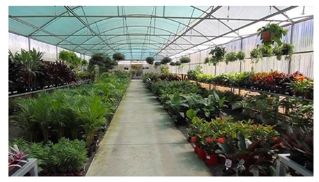
CASE STUDY AND NUMERICAL INVESTIGATION
Case Study
The present study represents a particular study of a
green item retailer's inventory system (the same case study is discussed by Mashud
et al. (2021)). In this greenhouse
farm, many agricultural products like vegetables, flowers, and fruits are
supplied to retailers. Since these items have the highest possibility to
deteriorate over time, retailers invested in preservation technologies to
control deterioration. A case study is presented in this section (Fig. 4) of a
greenhouse firm in Australia. They also invested in green technologies to
reduce carbon emissions from the environment.
Numerical Investigation
In the present model, an agreement is built between
the supplier and the retailer. The retailer gets an offer from a supplier that
he can pay the amount in equal installments and on
delivery, the remaining payment can be cleared up. Since it is a good deal for
the retailer, he agrees to this agreement Dye et al. (2007). The retailer
receives his ordering stock from the supplier by transport. This transport
system causes carbon emission, which is harmful to our environment. At ![]() , the
retailer gets his whole inventory after paying the remaining balance. In the
interval
, the
retailer gets his whole inventory after paying the remaining balance. In the
interval ![]() , the
retailer tries to accomplish the market’s demand. The demand of the model is
the joint function of selling price and inventory level, which is a realistic
demand pattern of the present business market Goyal
and Giri (2003). The inventory level
became zero at
, the
retailer tries to accomplish the market’s demand. The demand of the model is
the joint function of selling price and inventory level, which is a realistic
demand pattern of the present business market Goyal
and Giri (2003). The inventory level
became zero at ![]() because of
customer demand and product deterioration. For optimal results, the retailer
invests in preservation technologies which are required for the product to
maintain their quality for a long time. The above-defined model is considered
under the effect of inflation. Most of the time, inflation increases the cost
of the retailer, but it has to be taken as one of the realistic parts of the
inventory system Skouri and
Papachristos (2003), Bhunia
and Maiti (1998).
because of
customer demand and product deterioration. For optimal results, the retailer
invests in preservation technologies which are required for the product to
maintain their quality for a long time. The above-defined model is considered
under the effect of inflation. Most of the time, inflation increases the cost
of the retailer, but it has to be taken as one of the realistic parts of the
inventory system Skouri and
Papachristos (2003), Bhunia
and Maiti (1998).
A numerical study is investigated in this part to
validate the present paper. Mathematics 12.0 is used to solve both considered
models.
Case-1 (Considering Preservation Technology)
The following parameters have been considered for the
numerical example:
·
Ordering cost: ![]()
·
Selling price: ![]()
·
Holding cost parameters: ![]()
·
Inflation parameter: ![]()
·
Sensitivity parameter: ![]()
·
Deterioration parameter: ![]()
·
Fixed transportation cost: ![]()
·
Additional fuel cost: ![]()
·
Additional carbon emission cost: ![]()
·
Carbon emission cost: ![]()
·
Product's weight ![]()
·
Variable transportation cost: ![]()
·
Distance ![]()
·
Number of trips ![]()
·
Total number of installments
![]()
·
Remaining part of the amount on delivery ![]()
·
Lead time ![]()
·
Capital interest charge ![]()
·
Total purchase cost: ![]()
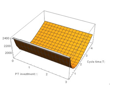
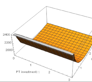
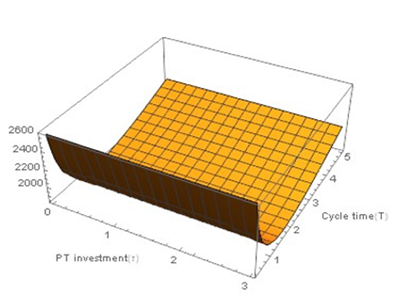
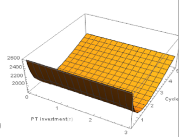
On solving Eq. (15), we noted the optimum values of PT
investment ![]() , cycle
time
, cycle
time ![]() and total cost
and total cost ![]() . Fig.
represents the convexity of the cost function regarding decision variables
. Fig.
represents the convexity of the cost function regarding decision variables ![]() and
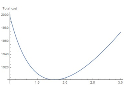
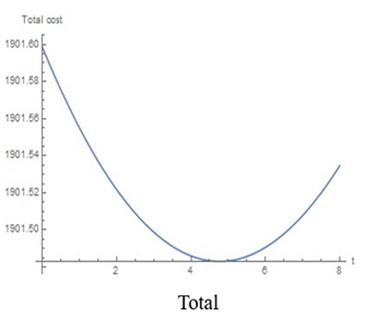
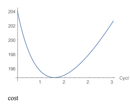
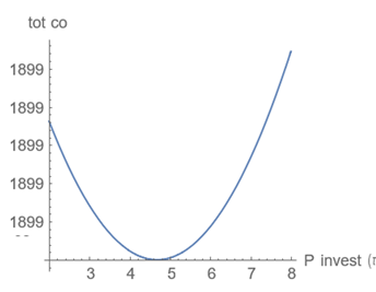
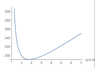
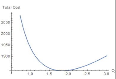
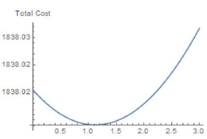
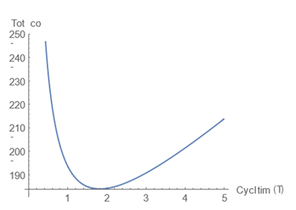
and ![]() . Fig.7. 6
and Fig. 7 show the convexity of the total cost function relative to individual
decision variables
. Fig.7. 6
and Fig. 7 show the convexity of the total cost function relative to individual
decision variables ![]() and
and ![]() .
.
No Preservation Technology (![]() )
)
Investment in preservation technologies is important
for most of the products to control deterioration, but there are many products
that do not require preservation technology investment to hold their quality
for their life period. Such products include stationery items like pens,
scales, electronic items, etc. We modified our model without considering the PT
investment (i.e., ![]() ). The
above-mentioned example is investigated for this case. The following optimum
solutions are obtained: cycle time
). The
above-mentioned example is investigated for this case. The following optimum
solutions are obtained: cycle time ![]() and the total cost is obtained as
and the total cost is obtained as ![]() . Fig. 8
shows the convexity of the cost function.
. Fig. 8
shows the convexity of the cost function.
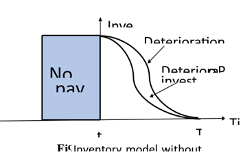
No Advance Payment
If an advance payment scheme is not applied, we
modified our model with the assumptions of preservation investment with no
advance payment, and the corresponding situation is shown in Fig. 9. To examine
this condition, we omit the cyclic capital cost in the total cost function. The
same example is again investigated in this scenario. The optimum values are as
follows: preservation investment parameter ![]() , cycle
time
, cycle
time ![]() and the total cost is obtained as
and the total cost is obtained as ![]() . Fig. 10
shows the convex nature of the total cost function concerning decision
variables
. Fig. 10
shows the convex nature of the total cost function concerning decision
variables ![]() and
and ![]() . Fig. 11
and Fig. 12 present the convex behavior of total cost relative to independent
decision variables
. Fig. 11
and Fig. 12 present the convex behavior of total cost relative to independent
decision variables ![]() and
and ![]() .
.
Full Advance Payment
Paying full product payment in a single installment is not possible for most retailers, but some
retailers can pay their whole amount in a single installment
or advance payment. We can modify our proposed model for this scenario also.
Putting ![]() and
and ![]() in Eq.
(15), we consider the same example to investigate for this part. With
in Eq.
(15), we consider the same example to investigate for this part. With ![]() and
and ![]() , we noted
the optimum values of PT investment
, we noted
the optimum values of PT investment ![]() , cycle
time
, cycle
time ![]() and total cost
and total cost ![]() .
.
Case-2 (Considering Both Preservation and Green Technology)
In the extension of this model, we optimize the total
cost given in Eq. (16). We considered the same examples mentioned above with
additional parameters such as ![]() ,
, ![]() , and
, and ![]() . We noted
the optimum values as PT investment
. We noted
the optimum values as PT investment ![]() , cycle
time
, cycle
time ![]() and total cost
and total cost ![]() . The
optimum values show that investment in green technology for controlling carbon
emission is much more beneficial for retailers as it increases total cost while
it increases the cycle length of the inventory system (see Fig. 13 for
convexity of the cost function). The convexity of the cost function relative to
individual decision variables
. The
optimum values show that investment in green technology for controlling carbon
emission is much more beneficial for retailers as it increases total cost while
it increases the cycle length of the inventory system (see Fig. 13 for
convexity of the cost function). The convexity of the cost function relative to
individual decision variables ![]() and
and ![]() can be
seen in Fig. 14 and Fig. 15.
can be
seen in Fig. 14 and Fig. 15.
No preservation technology (![]() )
)
We modified the present model without taking
preservation technology investment, i.e., ![]() . The
following optimum solutions are obtained: cycle time
. The
following optimum solutions are obtained: cycle time ![]() years and
the total cost is obtained as
years and
the total cost is obtained as ![]() . The
convexity of the total cost function for decision variables
. The
convexity of the total cost function for decision variables ![]() and
and ![]() is shown
in Fig. 16.
is shown
in Fig. 16.
Without advance payment
The optimum value for this case is as follows:
preservation investment parameter ![]() , cycle
time
, cycle
time ![]() years, and
the total cost is obtained as
years, and
the total cost is obtained as ![]() (See Fig.
17 for convexity of cost function concerning decision variables
(See Fig.
17 for convexity of cost function concerning decision variables ![]() and
and ![]() ).
).
Full advance payment
Full advance payment is another real scenario in the
business world. We noted the optimum values in this case as follows:
preservation investment ![]() / unit,
cycle time
/ unit,
cycle time ![]() years, and
total cost
years, and
total cost ![]() .
.
|
Figure 4
|
|
Figure 4 A Vegetable Firm with the Deteriorating Product |
|
Figure 5
|
|
Figure 5 Convexity
of the Total Cost Function |
|
Figure 6
|
|
Figure 6 Total Cost Function V/S PT Investment Cost |
|
Figure 7
|
|
Figure 7 Total
Cost Function V/S Cycle Time |
|
Figure 8
|
|
Figure 8 Convexity
of the Cost Function |
|
Figure 9
|
|
Figure 9 Inventory
Model Without Advance Payment |
|
Figure 10
|
|
Figure 10 Convexity
of the Cost Function |
|
Figure 11
|
|
Figure 11 Total
Cost Function V/S PT Investment Cost |
|
Figure 12
|
|
Figure 12 Total
Cost Function V/S Cycle Time |
|
Figure 13
|
|
Figure 13 Convexity
of the Cost Function |
|
Figure 14
|
|
Figure 14 Total
Cost Function V/S Cycle Time |
|
Figure 15
|
|
Figure 15 Total
Cost Function V/S Pt Investment Cost |
|
Figure 16
|
|
Figure 16 Convexity
of the Cost Function |
|
Figure 17
|
|
Figure 17 Convexity
of the Cost Function |
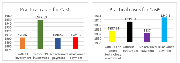
RESULTS SUMMARY
Many cases have been discussed in section 6. Fig.7.18.
shows the crisp summary of considered cases. The left part of Fig.7.18.
portrays the outcomes of Case-1 while the right side shows the results for
Case-2. It is noted that investment in GT would be beneficial for all subcases
as it always decreases the total cost Covert
and Philip (1973). The cost in the
first sub-case of Case-2 is 3.43% less than of Case1. The cost in the second
sub-case of Case-2 is 5.85% less than of Case-1. Similarly, the costs in the
remaining sub-cases of Case-2 are 3.41% and 3.29% than of Case-1 respectively.
‘No advance payment’ shows better results and it provided the lowest cost in
both cases but in an actual situation of an inventory structure, it is not
quite possible. In the pandemic of COVID-19, advance payment would be necessary
between supplier and retailer relationship Van der Veen, B. (1967), Naddor (1966). Sometimes advance
payment option helps the payer in the cancelation of the order in opposite
circumstances. Although, the overall system cost in the case of full advance
payment is 0.073% higher than the case of no advance payment for Case-1 while
this value is noted as 0.18% for Case-2. The total cost in the case of
preservation and green investment is 5.96% less than in the case of neither
preservation investment nor green investment Cambini and Martein (2009), Shah and Shah (2014).
|
Figure 18
|
|
Figure 18 Chart Summary for Special Cases |
|
Table 2 |
|
Table 2 Sensitivity Analysis for Case-1 |
|||||||
|
Parameter |
% Change |
τ |
T (with tech) |
TC* |
T (without tech) |
TC** |
(TC**−TC*) % |
|
c |
-20 |
12.8808 |
1.9105 |
1920.24 |
1.86122 |
1920.93 |
0.03 |
|
c |
-10 |
9.63547 |
1.84986 |
1933.58 |
1.8155 |
1933.99 |
0.02 |
|
c |
10 |
3.78761 |
1.74547 |
1959.04 |
1.73359 |
1959.1 |
0.003 |
|
c |
20 |
1.13095 |
1.70003 |
1971.22 |
1.69669 |
1971.23 |
0.0005 |
|
pᶜ |
-20 |
5.66138 |
1.80247 |
1923.25 |
1.78347 |
1923.28 |
0.0015 |
|
pᶜ |
-10 |
6.13973 |
1.79881 |
1934.88 |
1.77826 |
1935.03 |
0.007 |
|
pᶜ |
10 |
7.08536 |
1.79155 |
1958.12 |
1.76797 |
1958.33 |
0.01 |
|
pᶜ |
20 |
7.55274 |
1.78795 |
1969.73 |
1.76286 |
1969.97 |
0.012 |
|
p |
-20 |
108.644 |
0.852451 |
9408.85 |
0.762942 |
9737.94 |
3.49 |
|
p |
-10 |
78.5706 |
1.08203 |
5735.93 |
0.950973 |
5921.82 |
3.24 |
|
p |
10 |
– |
– |
– |
63.2028 |
– |
– |
|
p |
20 |
– |
– |
– |
63.1995 |
– |
– |
|
r |
-20 |
6.80433 |
1.84824 |
1891.48 |
1.80221 |
1938.2 |
2.47 |
|
r |
-10 |
5.73972 |
1.82868 |
1895.85 |
1.7846 |
1942.46 |
2.45 |
|
r |
10 |
3.68887 |
1.79159 |
1904.45 |
1.75098 |
1950.87 |
2.43 |
|
r |
20 |
2.7 |
1.77397 |
1908.68 |
1.74541 |
1955.02 |
2.42 |
|
w |
-20 |
2.4876 |
1.86984 |
1596.52 |
1.88924 |
1634.48 |
2.37 |
|
w |
-10 |
8.2475 |
1.88338 |
1748.62 |
1.8274 |
1790.85 |
2.4 |
|
w |
10 |
11.5949 |
1.78373 |
2050.62 |
1.72497 |
2102.06 |
2.52 |
|
w |
20 |
17.9468 |
1.75982 |
2200.34 |
1.68199 |
2257.04 |
2.57 |
|
h₁ |
-20 |
4.71157 |
1.81007 |
1900.07 |
1.77331 |
1946.58 |
2.44 |
|
h₁ |
-10 |
4.70663 |
1.80994 |
1900.12 |
1.77331 |
1946.63 |
2.44 |
|
h₁ |
10 |
4.69675 |
1.80955 |
1900.22 |
1.77298 |
1946.73 |
2.44 |
|
h₁ |
20 |
4.69181 |
1.80995 |
1900.27 |
1.77287 |
1946.78 |
2.44 |
|
h₂ |
-20 |
4.70809 |
1.80975 |
1900.18 |
1.77304 |
1946.7 |
2.44 |
|
h₂ |
-10 |
4.70489 |
1.80988 |
1900.16 |
1.77314 |
1946.67 |
2.44 |
|
h₂ |
10 |
4.69849 |
1.80975 |
1900.18 |
1.77304 |
1946.7 |
2.44 |
|
h₂ |
20 |
4.69529 |
1.80968 |
1900.2 |
1.77298 |
1946.71 |
2.44 |
|
|
|
Table 3 |
|
Table 3 Sensitivity Analysis for Case-2 |
||||||
|
arameter |
% Change |
Τ |
T |
TC* |
TC** |
(TC**−TC*) % |
|
c |
-20 |
7.20452 |
1.95133 |
1813.27 |
1920.24 |
5.89 |
|
c |
-10 |
4.05768 |
1.8913 |
1825.83 |
1933.58 |
5.9 |
|
c |
10 |
4.1736 |
1.78756 |
1849.83 |
1959.04 |
5.9 |
|
c |
20 |
2.2802 |
1.74266 |
1861.34 |
1971.22 |
5.9 |
|
pᶜ |
-20 |
0.075927 |
1.84491 |
1814.5 |
1923.25 |
5.99 |
|
pᶜ |
-10 |
0.601824 |
1.84094 |
1826.26 |
1934.88 |
5.94 |
|
pᶜ |
10 |
1.64037 |
1.83309 |
1849.75 |
1958.12 |
5.89 |
|
pᶜ |
20 |
1.66204 |
1.8315 |
1878.82 |
1969.73 |
5.17 |
|
p |
-20 |
105.359 |
0.86778 |
8976.91 |
9408.85 |
4.52 |
|
p |
-10 |
75.219 |
1.10077 |
5487.7 |
5735.93 |
4.52 |
|
p |
10 |
50.472 |
1.1016 |
4287.1 |
4529.12 |
5.64 |
|
p |
20 |
18.725 |
1.10273 |
3268.25 |
3451.37 |
5.6 |
|
r |
-20 |
3.30135 |
1.87741 |
1829.18 |
1891.48 |
3.4 |
|
r |
-10 |
2.19802 |
1.85683 |
1833.62 |
1895.85 |
3.39 |
|
r |
10 |
0.0756 |
1.81787 |
1842.35 |
1904.45 |
3.37 |
|
r |
20 |
0.0741 |
1.78155 |
1850.89 |
1908.68 |
3.12 |
|
w |
-20 |
5.8129 |
1.89497 |
1550.08 |
1596.52 |
2.99 |
|
w |
-10 |
7.3679 |
1.86463 |
1694.54 |
1748.86 |
3.2 |
|
w |
10 |
8.01778 |
1.81173 |
1980.64 |
2050.62 |
3.53 |
|
w |
20 |
14.3744 |
1.78852 |
2122.55 |
2200.34 |
3.66 |
|
h₁ |
-20 |
1.3313 |
1.83727 |
1837.91 |
1900.07 |
3.38 |
|
h₁ |
-10 |
1.12821 |
1.83714 |
1837.96 |
1900.12 |
3.38 |
|
h₁ |
10 |
1.11836 |
1.83687 |
1838.06 |
1900.22 |
3.38 |
|
h₁ |
20 |
1.11343 |
1.83673 |
1838.11 |
1900.27 |
3.38 |
|
h₂ |
-20 |
1.12977 |
1.83714 |
1837.98 |
1900.14 |
3.38 |
|
h₂ |
-10 |
1.12653 |
1.83707 |
1838 |
1900.16 |
3.38 |
|
h₂ |
10 |
1.12004 |
1.83693 |
1838.02 |
1900.18 |
3.38 |
|
h₂ |
20 |
1.11679 |
1.83686 |
1838.04 |
1900.2 |
3.38 |
|
m |
-20 |
0.50239 |
1.84169 |
1824.03 |
1886.25 |
3.41 |
|
m |
-10 |
0.81361 |
1.83934 |
1831.02 |
1893.21 |
3.39 |
|
m |
10 |
– |
– |
– |
1907.13 |
– |
|
m |
20 |
1.73799 |
1.83235 |
1851.98 |
1914.08 |
3.35 |
|
K |
-20 |
1.11438 |
1.83707 |
1837.81 |
– |
– |
|
K |
-10 |
1.11883 |
1.83704 |
1837.91 |
1900.12 |
3.38 |
|
K |
10 |
1.12773 |
1.83697 |
1838.11 |
1900.22 |
3.37 |
|
K |
20 |
1.13218 |
1.83694 |
1838.21 |
1900.27 |
3.37 |
|
n |
-20 |
1.12513 |
1.83699 |
1838.05 |
1900.19 |
3.38 |
|
n |
-10 |
1.12411 |
1.837 |
1838.03 |
1900.18 |
3.38 |
|
n |
10 |
1.12261 |
1.83701 |
1837.99 |
1900.16 |
3.38 |
|
n |
20 |
1.12205 |
1.83701 |
1837.98 |
1900.16 |
3.38 |
|
e₁ |
-20 |
3.7319 |
1.93211 |
1573.26 |
1619.77 |
7.53 |
|
e₁ |
-10 |
4.97424 |
1.88264 |
1706.17 |
1760.52 |
3.18 |
|
e₁ |
10 |
6.67235 |
1.79472 |
1968.93 |
2038.86 |
3.55 |
|
e₁ |
20 |
11.7591 |
1.7554 |
2099.04 |
2176.72 |
3.7 |
|
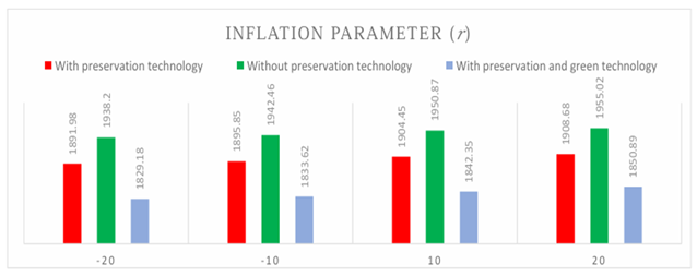
Figure 19
|
|
Figure 19 Pictorial View of Sensitivity Analysis of Inflation Parameter (R) |
|
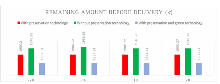
Figure 20
|
|
Figure 20 Pictorial View of Sensitivity Analysis Of (𝜎) |
|
Figure 21
|
|
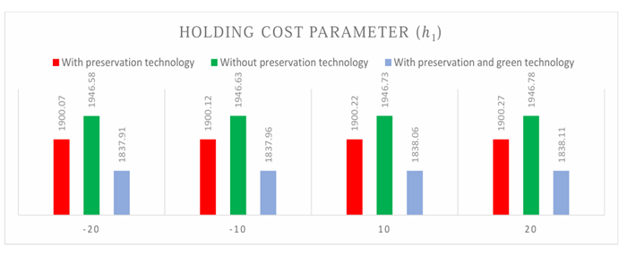
Figure 21 Pictorial View of Sensitivity Analysis of Holding
Cost Parameter (ℎ1) |
|
Figure 22
|
|
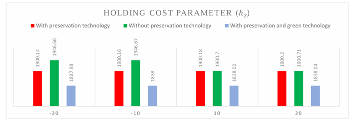
Figure 22 Pictorial View of Sensitivity Analysis of Holding
Cost Parameter (ℎ2) |
|
Figure 23
|
|
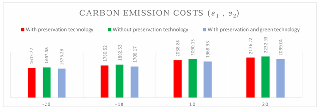
Figure 23 Pictorial View of Sensitivity Analysis of Carbon
Emission Costs (𝑒1, 𝑒2) |
|
Figure 24
|
|
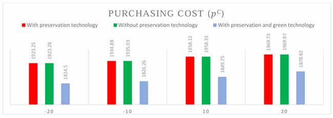
Figure 24 Pictorial View of Sensitivity Analysis of Purchasing
Cost Parameter (𝑝c) |
SENSITIVITY ANALYSIS
The model that is under use is based on several
fundamental parameters. The effects of such parameters in this section have
been studied, i.e. the effect and influence of changes in this
parameters, which in turn resulted to the occurrence of different
observations in an ideal solution to the two cases considered.
Case-1
The case of with and without PT investment is studied
in Table 2.
·
Increasing values of (, m, e_1, e_2,) and (d_s) increases the system cost of the model in both cases
with and without PT investment as they enhance the carbon emission and
transportation cost also. The average increment in total cost from without
preservation technology are 2.46%, 2.44%, 2.45%, 2.45%, and 0.075%,
respectively.
·
The increasing value of (r) increases the total cost
as it is an inflation factor. The retailer should always concern about
inflation for being a realistic situation. The average increment in total cost
from without preservation technology is 2.44% from the sensitivity of (r).
·
An increment in the value of (n) decreases the total
cost while it increases the time length of the system. The average increment in
total cost from without preservation technology is 2.44% from the sensitivity
of (n).
·
The total cost increases after the increment in (K)
and ( \sigma ). However, the higher cost is obtained
in the case of without preservation technology. The average increment in total
cost from without preservation technology is 2.44% and 2.57%, respectively.
·
Increasing parameter ( p )
decreases the total cost and increases the cycle length (T).
·
The increment ( p^* ) is not beneficial for the present inventory model. The
retailer is facing higher purchasing costs with time which leads to less
profit. The average increment in total cost from without preservation
technology is 2.44%.
·
Both the holding cost parameters (h_1) and (h_2) also
show the same negative impact as (p^*) shown. The average increment in total
cost from without preservation technology is 2.44% for both the holding cost
parameters.
Case-2
The case of with and without GT investment is examined
in Table 3.
·
The carbon emission factors (e_1) and (e_2) increases,
the total cost after the increment in their values. When the retailer does not
incorporate green technology, the higher carbon emission cost is noted. Figure 2 shows that the
average decrement in the total cost of without preservation technology and with
green technology is 5.87% from the sensitivity of carbon emission cost
parameters ![]() and
and ![]() .
.
·
The inflation parameter ![]() shows the
higher effect on total cost in the case of no green techniques. Fig. 19 shows
that the average decrement in the total cost of without preservation technology
and with green technology is 5.85% from the sensitivity of inflation parameter
shows the
higher effect on total cost in the case of no green techniques. Fig. 19 shows
that the average decrement in the total cost of without preservation technology
and with green technology is 5.85% from the sensitivity of inflation parameter ![]() . So, the
investment in green technology should be increased to compensate for the effect
of inflation.
. So, the
investment in green technology should be increased to compensate for the effect
of inflation.
·
The higher values of ![]() ,
, ![]() , and
, and ![]() have a
negative effect on the model. The cycle length of the retailer’s system
decreases while the total cost becomes higher.
have a
negative effect on the model. The cycle length of the retailer’s system
decreases while the total cost becomes higher.
·
When ![]() and
and ![]() increase,
the retailer has to face an immense total cost for less system cycle. From Fig.
20, it is observed that the average decrement in the total cost of without
preservation technology and with green technology is 6.05% from the sensitivity
of
increase,
the retailer has to face an immense total cost for less system cycle. From Fig.
20, it is observed that the average decrement in the total cost of without
preservation technology and with green technology is 6.05% from the sensitivity
of ![]() .
.
·
The higher value of several installments
![]() is
beneficial for the retailer. As
is
beneficial for the retailer. As ![]() escalates,
the time to pay the remaining amount also increases, which would help to run
the inventory system more conveniently.
escalates,
the time to pay the remaining amount also increases, which would help to run
the inventory system more conveniently.
·
![]() ,
, ![]() , and
holding cost parameters
, and
holding cost parameters ![]() and
and ![]() show the
negative effect on the retailer’s profit. It is reducing the cycle length of
the system while increasing the total cost. Fig. 21 and Fig. 22 show that the
average decrement in the total cost of without preservation technology and with
green technology is 5.91% and 4.65%, respectively, from the sensitivity of
holding cost parameters and
show the
negative effect on the retailer’s profit. It is reducing the cycle length of
the system while increasing the total cost. Fig. 21 and Fig. 22 show that the
average decrement in the total cost of without preservation technology and with
green technology is 5.91% and 4.65%, respectively, from the sensitivity of
holding cost parameters and ![]() ,
respectively. Fig. 24 shows that the average decrement in the total cost of
without preservation technology and with green technology is 5.66% from the
sensitivity of purchasing cost parameter
,
respectively. Fig. 24 shows that the average decrement in the total cost of
without preservation technology and with green technology is 5.66% from the
sensitivity of purchasing cost parameter ![]() .
.
MANAGERIAL INSIGHTS
The discussed model is developed around the retailer's
profit. The main highlights of the paper can be availed by firms to reduce the
total cost with less investment.
Most of the retailers can apply this model as the
proposed model dealt with a more realistic condition, inflation.
This model majorly helps greenhouse firms to control
the carbon emission by investing in the proposed green technology.
With the help of this model, the retailers can
comfortably understand when they are required to invest in preservation
technology or when to implement green technology, or when the investment in
both technologies is needed.
In COVID-19,
most of the suppliers can request the retailer for the advance payment to get
more profit, especially in the greenhouse business as there are more chances of
canceling the order due to its deteriorating behavior. The retailers pay less cost in the absence of
advance payments. The proposed advance payment scheme can be applied if the
retailers are incapable to pay an immense amount in a single installment.
An ideal demand rate is incorporated in this study
which is a composition of selling price and stock of the system. This increases
the importance of this model as more retailers can apply this model in their
business.
Transportation cost is one of the main costs which can
be handled wisely to maintain the profit of industry. With the help of this
study, a manager can simply estimate the transportation cost. If the retailer
has to transform all these outputs to a built-in function to prepare an excel
solver, then the proposed study can supply more benefits.
CONCLUSION
The economic order quantity system has been innovated
which suffers in nature in the given model. The green firm product retailer in
this model is investing in the preservation technology to cope with loss of the
product as a result of deterioration and in green technology to cope with the
carbon gas released in the process of transportation system. In the given
study, numerous variables have been taken into account when the information was
devoted to COVID-19 like the quality of the good, the method of payment, the
inclination to the demand, the price was lowered overall. The rate of demand
depends upon inventory and the selling price (which is a more realistic
condition). The cost of stock holding has been considered to be a linear output
of time (when it is assumed that the cost of stock holding is increasing with
time). This model is losing money away with time i.e. in this model an
inflation should be taking place. It gave various requirements on advance
payment by the supplier to the retailers. The optimal goal of the current paper
will be to streamline the cycle time and investment cost of system preserve
tech and green technology. This model passes through the different states that
lead to the conclusion that where there are no funds on the preservation and
green technologies effect on the increment in the total cost as it even adds to
the decrease in the cycle time. The aforementioned variables attributed to the
transportation system, i.e. the distance covered by the shipment, the weight of
the products and the conveyance emission, have been identified to be subject of
consideration by the retailers as they determine the increment and decrease of
the cost and cycle length of the system respectively.
The paper under consideration can be related to the
item or multi-item inventory system in trade credit policy that would bring it
closer to reality in further studies. Part of the contribution to this
prevailing literature would be in the form of rationing and backlogging. They
also can make various forms of deterioration on this proposed model to make the
model relatablev.
ACKNOWLEDGMENTS
None.
REFERENCES
Balaman, S.Y., and Selim, H. (2016). Sustainable Design of Renewable Energy Supply Chains Integrated with District Heating Systems: A Fuzzy Optimization Approach. ` Journal of Cleaner Production, 133, 863–885. https://doi.org/10.1016/j.jclepro.2016.06.001
Banerjee, S., Agrawal, S., and Gupta, R. (2018). Retailers Optimal Payment Decisions for Price-Dependent Demand Under Partial Advance Payment and Trade Credit in Different Scenarios Retailer’s Optimal Payment Decisions for Price-dependent Demand under Partial Advance Payment and Trade Credit in Different Scenarios. International Journal of Scientific Research Mathematical and Statistical Sciences, 5, 44–53. https://doi.org/10.26438/ijsrmss/v5i4.4453
Bhunia, A. K., and Maiti, M. (1998). Deterministic Inventory Model for Deteriorating Items with Finite Rate of Replenishment Dependent on Inventory level. Computers and Operations Research, 25(11), 997–1006. https://doi.org/10.1016/S0305-0548(97)00091-9
Cambini, A., and Martein, L. (2009). Generalized and optimization generalized convexity: Theory and Applications. Lect. Notes Econ. Math. Syst. 616, 1–262. https://doi.org/10.1007/978-3-540-70876-6
Chandra Das, S., Zidan, A. M., Manna, A. K., Shaikh, A. A., and Bhunia, A. K. (2020). An Application of Preservation Technology in Inventory Control System with Price Dependent Demand and Partial Backlogging. Alexandria Engineering Journal, 59(3), 1359–1369. https://doi.org/10.1016/j.aej.2020.03.006
Chang, C. T., Ouyang, L. Y., Teng, J. T., Lai, K. K., and Cárdenas-Barrón, L. E. (2019). Manufacturer’s Pricing and Lot-Sizing Decisions for Perishable Goods Under Various Payment Terms by a Discounted Cash Flow Analysis. International Journal of Production Economics, 218, 83–95. https://doi.org/10.1016/j.ijpe.2019.04.039
Chen, L., Cai, W., and Ma, M. (2020). Decoupling or Delusion? Mapping Carbon Emission Per Capita Based on the Human Development Index in Southwest China. Science of the Total Environment, 741, 138722. https://doi.org/10.1016/j.scitotenv.2020.138722
Chen, L., Chen, X., Keblis, M. F., and Li, G. (2019). Optimal pricing and replenishment policy for deteriorating inventory under stock-level-dependent, time-varying and price-dependent demand. Computers and Industrial Engineering, 135, 1294–1299. https://doi.org/10.1016/j.cie.2018.06.005
Covert, R. P., and Philip, G. C. (1973). An Eoq Model for Items with Weibull distribution deterioration. AIIE Transactions, 5(4), 323–326. https://doi.org/10.1080/05695557308974918
Das, S.C., Manna, A.K., Rahman, M.S., Shaikh, A.A., and Bhunia, A.K. (2021). An Inventory Model for Noninstantaneous Deteriorating Items with Preservation Technology and Multiple Credit Periods-Based Trade Credit Financing Via Particle Swarm Optimization. Soft Comput. 25, 5365–5384. https://doi.org/10.1007/s00500-020-05535-x
Datta, T. K. (2017). Effect of Green Technology Investment on a Production-Inventory System with Carbon Tax. Advances in Operations Research, 2017. https://doi.org/10.1155/2017/4834839
Datta, T. K., Nath, P., and Dutta Choudhury, K. (2020). A Hybrid Carbon Policy Inventory Model with Emission Source-Based Green Investments. OPSEARCH, 57(1), 202–220. https://doi.org/10.1007/s12597-019-00430-y
Dye, C. Y. (2013). The Effect of Preservation Technology Investment on a Non-Instantaneous Deteriorating Inventory Model. Omega (United Kingdom), 41(5), 872–880. https://doi.org/10.1016/j.omega.2012.11.002
Dye, C. Y., Ouyang, L. Y., and Hsieh, T. P. (2007). Deterministic Inventory Model for Deteriorating Items with Capacity Constraint and Time-Proportional Backlogging Rate. European Journal of Operational Research, 178(3), 789–807. https://doi.org/10.1016/j.ejor.2006.02.024
Dye, C. Y., and Hsieh, T. P. (2013). A Particle Swarm Optimization for Solving Lot-Sizing Problem with Fluctuating Demand and Preservation Technology Cost Under Trade Credit. Journal of Global Optimization, 55(3), 655–679. https://doi.org/10.1007/s10898-012-9950-z
Gaur, A., Tayal, S., and Singh, S.R. (2020). Replenishment Policy for Deteriorating Items with Trade Credit and Allowable Shortages Under Inflationary Environment. Int. J. Process Manag. Benchmarking 10, 462. https://doi.org/10.1504/ijpmb.2020.10027580
Ghare, P.M. and Schrader, G.F. (1963) A Model for an Exponential Decaying Inventory. Journal of Industrial Engineering, 14, 238-243. - References - Scientific Research Publishing. (n.d.).
Giri, B. C., Pal, H., and Maiti, T. (2017). A Vendor-Buyer Supply Chain Model for Time-Dependent Deteriorating item with Preservation Technology Investment. International Journal of Mathematics in Operational Research, 10(4), 431–449. https://doi.org/10.1504/IJMOR.2017.084158
Goyal, S. K., and Giri, B. C. (2003). The Production-Inventory Problem of a Product with Time Varying Demand, Production and Deterioration Rates. European Journal of Operational Research, 147(3), 549–557. https://doi.org/10.1016/S0377-2217(02)00296-5
Hsieh, T. P., and Dye, C. Y. (2010). Pricing and Lot-Sizing Policies for Deteriorating Items with Partial Backlogging Under Inflation. Expert Systems with Applications, 37(10), 7234–7242. https://doi.org/10.1016/j.eswa.2010.04.004
Hsieh, T. P., and Dye, C. Y. (2017). Optimal Dynamic Pricing for Deteriorating Items with Reference Price Effects when Inventories Stimulate Demand. European Journal of Operational Research, 262(1), 136–150. https://doi.org/10.1016/j.ejor.2017.03.038
Jawla, P., and Singh, S.R. (2016). A Reverse Logistic Inventory Model for Imperfect Production Process with Preservation Technology Investment Under Learning and Inflationary Environment. Uncertain Supply Chain Manag. 4, 107–122. https://doi.org/10.5267/j.uscm.2015.12.001
Khanna, A., Priyamvada, and Jaggi, C. K. (2020). Optimizing Preservation Strategies for Deteriorating Items with Time-Varying Holding Cost and Stock-Dependent Demand. Yugoslav Journal of Operations Research, 30(2), 237–250. https://doi.org/10.2298/YJOR190215003K
Kumar, M., Chauhan, A., Singh, S.J., and Sahni, M. (2020). An Inventory Model on Preservation Technology with Trade Credits Under Demand Rate Dependent on Advertisement, Time and Selling Price. Univers. J. Account. Financ. 8, 65–74. https://doi.org/10.13189/ujaf.2020.080302
Lashgari, M., Taleizadeh, A. A., and Ahmadi, A. (2016). Partial Up-Stream Advanced Payment and Partial Down-Stream Delayed Payment in a Three-Level Supply Chain. Annals of Operations Research, 238(1–2), 329–354. https://doi.org/10.1007/s10479-015-2100-5
Li, R., Skouri, K., Teng, J. T., and Yang, W. G. (2018). Seller’s Optimal Replenishment Policy and Payment Term Among Advance, Cash, and Credit Payments. International Journal of Production Economics, 197, 35–42. https://doi.org/10.1016/j.ijpe.2017.12.015
Lou, G. X., Xia, H. Y., Zhang, J. Q., and Fan, T. J. (2015). Investment Strategy of emission-reduction technology in a supply Chain. Sustainability (Switzerland), 7(8), 10684–10708. https://doi.org/10.3390/su70810684
Mashud, A.H.M., Roy, D., Daryanto, Y., Chakrabortty, R.K., and Tseng, M.L. (2021). A Sustainable Inventory Model with Controllable Carbon Emissions, Deterioration and advance payments. J. Clean. Prod. 296, 126608. https://doi.org/10.1016/j.jclepro.2021.126608
Mishra, U., Wu, J.Z., Tsao, Y.C., and Tseng, M.L. (2020). Sustainable Inventory System with Controllable Noninstantaneous Deterioration and Environmental Emission Rates. J. Clean. Prod. 244. https://doi.org/10.1016/j.jclepro.2019.118807
Naddor, E. (1966). Dimensions in Operations Research. Operations Research, 14(3), 508–514. https://doi.org/10.1287/opre.14.3.508
Pando, V., San-José, L. A., García-Laguna, J., and Sicilia, J. (2013). An Economic Lot-Size Model with Non-Linear Holding Cost Hinging on Time and Quantity. International Journal of Production Economics, 145(1), 294–303. https://doi.org/10.1016/j.ijpe.2013.04.050
Pervin, M., Roy, S.K., and Weber, G.W. (2020). Deteriorating Inventory with Preservation Technology Under Price and Stock-Sensitive Demand. J. Ind. Manag. Optim. 16, 1585–1612. https://doi.org/10.3934/jimo.2019019
Sarkar, B., Cárdenas-Barrón, L. E., Sarkar, M., and Singgih, M. L. (2014). An Economic Production Quantity Model with Random Defective Rate, Rework Process and Backorders for a Single Stage Production System. Journal of Manufacturing Systems, 33(3), 423–435. https://doi.org/10.1016/j.jmsy.2014.02.001
Shah, N., Rabari, K., and Patel, E. (2020). Inventory and Preservation Investment for Deteriorating System with Stock-Dependent Demand and Partial Backlogged Shortages. Yugosl. J. Oper. Res. 38–38. https://doi.org/10.2298/yjor200217038s
Shah, N.H., and Shah, A.D. (2014). Optimal Cycle Time and Preservation Technology Investment for Deteriorating Items with Price-Sensitive Stock-Dependent emand under inflation, in: Journal of Physics: Conference Series. Institute of Physics Publishing. https://doi.org/10.1088/1742-6596/495/1/012017
Shi, Y., Zhang, Z., Chen, S.C., Cárdenas-Barrón, L.E., and Skouri, K. (2020). Optimal Replenishment Decisions for Perishable Products Under Cash, Advance, and Credit Payments Considering Carbon Tax Regulations. Int. J. Prod. Econ. 223, 107514. https://doi.org/10.1016/j.ijpe.2019.09.035
Singh, S. R., Khurana, D., and Tayal, S. (2016). An Economic Order Quantity Model for Deteriorating Products Having Stock Dependent Demand with Trade Credit Period and Preservation Technology. Uncertain Supply Chain Management, 4(1), 29–42. https://doi.org/10.5267/j.uscm.2015.8.001
Skouri, K., and Papachristos, S. (2003). Four Inventory Models for Deteriorating Items with Time Varying Demand and Partial Backlogging: A Cost Comparison. Optimal Control Applications and Methods, 24(6), 315–330. https://doi.org/10.1002/oca.734
Taleizadeh, A. A., Pentico, D. W., Jabalameli, M. S., and Aryanezhad, M. (2013). An Economic Order Quantity Model with Multiple Partial Prepayments and Partial Backordering. Mathematical and Computer Modelling, 57(3–4),311–323. https://doi.org/10.1016/j.mcm.2012.07.002
Teng, J. T., Cárdenas-Barrón, L. E., Chang, H. J., Wu, J., and Hu, Y. (2016). Inventory Lot-Size Policies for Deteriorating Items with Expiration Dates and Advance Payments. Applied Mathematical Modelling, 40(19–20), 8605–8616. https://doi.org/10.1016/j.apm.2016.05.022
Tripathi, R.P., Singh, D., and Aneja, S., (2018). Inventory Models for Stock-Dependent Demand and Time Varying Holding Cost Under Different Trade Credits. Yugosl. J. Oper. Res. 28, 139–151. https://doi.org/10.2298/YJOR160317018T
Van der Veen, B. (1967). Introduction to the Theory of Operational Research. In Introduction to the Theory of Operational Research. Springer Berlin Heidelberg. https://doi.org/10.1007/978-3-662-42424-7
Wahab, M. I. M., Mamun, S. M. H., and Ongkunaruk, P. (2011). EOQ Models for a Coordinated Two-Level International Supply Chain Considering Imperfect Items and Environmental Impact. International Journal of Production Economics, 134(1), 151–158. https://doi.org/10.1016/j.ijpe.2011.06.008
Wu, J., Teng, J.T., and Chan, Y.L. (2018). Inventory Policies for Perishable Products with Expiration Dates and Advancecash-Credit Payment Schemes. Int. J. Syst. Sci. Oper. Logist. 5, 310–326. https://doi.org/10.1080/23302674.2017.1308038
Yang, C. Te, Dye, C. Y., and Ding, J. F. (2015). Optimal Dynamic Trade Credit and Preservation Technology Allocation for a Deteriorating Inventory Model. Computers and Industrial Engineering, 87, 356–369. https://doi.org/10.1016/j.cie.2015.05.027
Yu, L. C., and Hui, H. Y. (2008). An Empirical Study on Logistics Service Providers’ Intention to Adopt Green Innovations. Journal of Technology Management and Innovation, 3(1), 17–26.
Zauberman, G., Ronen, R., Akerman, M., Weksler, A., Rot, I., and Fuchs, Y. (1991). Post-Harvest Retention of the Red Colour of Litchi Fruit Pericarp. Scientia Horticulturae, 47(1–2), 89–97. https://doi.org/10.1016/0304-4238(91)90030-3
Zulu, K., Singh, R.P., and Shaba, F.A., (2020). Environmental and Economic Analysis of Selected Pavement Preservation tReatments. Civ. Eng. J. 6, 210–224. https://doi.org/10.28991/cej-2020-03091465
|
|
 This work is licensed under a: Creative Commons Attribution 4.0 International License
© IJETMR 2014-2026. All Rights Reserved.