ECONOMIC DESIGN OF PIPE-NOZZLE DISCHARGE LINES DELIVERING FREE JETS

 

Mohamed M. M. Amin ¹, Medhat M. H. ElZahar ²

 

¹ Professor of Hydraulics, Civil Engineering Department, Faculty of Engineering, Port Said University, Port Said, Egypt

² Associate Professor of Sanitary and Environmental Engineering, Department of Civil Engineering, Faculty of Engineering, Port Said University, Port Said, Egypt

 

1. INTRODUCTION

The pipe-nozzle discharge lines are known for a wide range of applications in practice, they are generally used to have a high-velocity water jet that can be used for firefighting, mining, and power developments (the impulse turbines) Featherstone and El-Jumaily (1983), Streeter and Wylie (1985), Sharp (1985). Most of the studies are based on hydraulic considerations, and in this study, an analytical solution has been reached using a derivative method associated with the economic considerations and comparison requirements Simon (1987), Somaida (1994), Somaida et al. (2011), Somaida et al. (2012). Little is found in the literature concerning the present problem. Most of the previous studies are directed toward having the maximum power of the jet delivered from the nozzle. However, the present study is based on economic considerations satisfying the choosing of the pipe-nozzle diameter ratio leading to the minimum cost of the discharge line. This will be presented within the scope here. However, an analytical solution is derived to solve the problem with comparison requirements John et. al. (2011), Mazzoleni (1994), Joseph et al. (2010), Somaida et al. (2013).

In practice, pipe nozzles are widely used in many water and wastewater engineering applications, such as irrigation systems, water supply, and wastewater system arrangements Wright et al. (2003), Poeck (2008). Common applications of nozzles in water and wastewater treatment systems are as follows: Koirala et al. (2021), BETE for Nozzle Performance Engineering (2022):

·        Evaporative disposal, such as disposal of excess water/chemical solution through evaporation, usually over a large pond.

·        Foam control, Spray nozzles to break up foam that can cause tank overflow, poor drainage, or other problems.

·        Mixing and blending tank contents, homogenizing sediment off the tank bottom to aid in transportation and filtration, sweeping solids across the bottom of the tank, and preventing thermal stratification.

·        Filter nozzles, which can be installed in both open and closed filters, to ensure maximum efficiency with minimum head losses Wright (2003), BETE for Nozzle Performance Engineering (2022).

·        Also, water jet lines and nozzles are used for sewer cleaning Medan et al. (2017).

There are analytical methods for the development of comprehensive costing dealing with the economic sizes of any pipeline Sharp (1985). This can be applied to the present problem, where the pipeline ends with a nozzle acting as a gravity main and should have the optimum diameter ratio Somaida et al. (1994), Somaida et al. (2011), Somaida et al. (2012), Somaida et al. (2013). Poeck et al. (2008), studied a performance evaluation of various nozzle designs for waterjet scaling in underground excavations. Design and optimization of discharge pipelines delivering free jets are of high concern in industry based on economic considerations Renjie (2020), Schwartzentruber et al. (2016).

 

2. MATERIALS AND METHODS

2.1. Minor nozzle loss

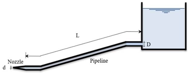
It is usually considered that for pipe of length longer than 1000 diameter (L/D>1000), the error incurred by neglecting minor losses is less than that inherent in selecting the value of friction factor F Joseph et al. (2010). In the case of an approach pipe ending with a nozzle, Figure 1, which has a known assumed loss coefficient, the head loss as associated with the high issuing velocity head and is therefore not as minor loss. But, in the present study, it is suggested that the minor loss of the nozzle may be expressed in terms of the equivalent length of approach pipe (L_e), that has the same head loss for the same discharge delivered from the nozzle De Cock (2017),  Radkevich et al. (2021), or

 

                                                             Equation 1

 

Where F = friction factor of approach pipe, L_e = equivalent length of pipe, V_P = velocity of flow in approach pipe, D = diameter of approach pipe, g = acceleration of gravity, K = loss coefficient of minor loss due to nozzle, V_J = absolute velocity of the jet, and d = diameter of nozzle opening (diameter of jet).

Note that from continuity equation,

 

                                                  Equation 2

 

Therefore, the total length of the pipe will be:

 

                                                                             Equation 3

 

However, the solution will be built around the friction factor of the approach pipe, rather than minor loss of the nozzle.

Figure 1

                                                                    

Figure 1 Pipe-Nozzle Discharge Line

 

2.2.  Pipe-nozzle discharge line cost

The pipe cost C_P is given by, Sharp (1985)

 

                                                                                                Equation 4

 

Where, a = pipe cost function and x = pipe cost exponent.

However, considering the pipe cost C_P of the pipe-nozzle discharge line, the equation of total pipe cost will be given by:

 

                                                                Equation 5

 

Where, K = loss coefficient of the nozzle, which is known by , where C_v = coefficient of velocity in the nozzle.

 

2.3. Derivative optimum for D/d ratio

In order to obtain the optimum D/d ratio, use the derivative method except that the cost gradient will be relative to the diameter of the approach pipe D, because the pipe now forms a major part of the scheme. However, for minimum pipe cost, differentiate Equation 5, with respect to D, and equate to zero, with the following assumptions:

1)     Constant diameter of nozzle opening d.

2)     Turbulent flow conditions and Reynold’s number ranges from 10⁵ to 10⁶, where the loss coefficient of the nozzle is relatively constant, without serious error, Joseph et al. (2010).

3)     Variable coefficient of friction.

Differentiate Equation 5 with respect to D and equate to zero, then:

 

          Equation 6

 

Put Equation 6 in the following form:

 

 

                                       Equation 7

 

The partial in the L.H.S. of Equation 7,  can be written in the form: or , However,  Equation 7, can take the form:

 

                                                                                 Equation 8

 

The form  can be evaluated from Von Karman formula for F: .

Introducing the diameter ratio, B , or , ؞    

Or . The term    in this equation is constant.

Differentiate F in this equation with respect to d,

؞         , or

Substitute by  in  Equation 8,

                                             Equation 9

 

Put the diameter ratio , in Equation 9 and rearrange for B, then:

 

                                         Equation 10

 

Where K is the minor loss coefficient of the nozzle = , since , Streeter and  Wylie (1985) and C is the flow coefficient of the nozzle. However, the diameter ratio D/d depends on friction factor F of approach pipe, loss coefficient of nozzle K, relative distance L/D, and pipe cost exponent x.  Equation 10 can be solved by trial and error.

 

2.4. Illustrative example

In the present illustrative example, the following data are given L = 20, D = 0.1m, relative distance L/D = 200, relative roughness e/D = 0.02 (F = 0.05). In view of the pipe cost exponent x, it was taken 0.45 by Featherstone and El-Jumaily (1983) and 1.03 by Somaida et al. (2012), However, it is taken 2.5 in the present study. The values of C at different D/d are evaluated using the following equation, which is evaluated by linear regression analysis of the data concerning the flow ratio C and the diameter ratio  being interpreted from Streeter and Wylie (1985)(“Fig. 8.16”, P. 467).

 

                                                                                            Equation 11

 

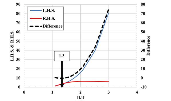
The results obtained by solving Equation 10 by trial and error as shown in Table 1.

Graphical solution of Equation 10 based on minimum pipe cost is shown in Figure 2. This figure and Table 2 show that, the solution of Equation 10 is satisfying at average value of D/d = 1.3.

Table 1

Table 1 Solving Equation 10 by Trial and Error at Different D/d for the Illustrative Example (L/D = 200 and F=0.05)
B (D/d)	C	Cv	K	L.H.S.	R.H.S.	Difference
1.1	0.8991	0.5062	2.9027	1.464	1.0260	0.4381
1.2	0.8919	0.6418	1.4279	2.074	2.0856	-0.0120
1.3	0.8854	0.7137	0.9630	2.856	3.0926	-0.2365
1.4	0.8794	0.7563	0.7483	3.842	3.9798	-0.1382
1.5	0.8738	0.7827	0.6321	5.063	4.7112	0.3513
1.6	0.8686	0.7996	0.5640	6.554	5.2800	1.2736
1.7	0.8638	0.8104	0.5226	8.352	5.6993	2.6528
1.8	0.8593	0.8173	0.4970	10.498	5.9919	4.5057
1.9	0.8550	0.8215	0.4817	13.032	6.1831	6.8490
2	0.8510	0.8239	0.4730	16	6.2963	9.7037
2.1	0.8472	0.8251	0.4689	19.448	6.3511	13.0970
2.5	0.8337	0.8229	0.4766	39.063	6.2485	32.8140
2.55	0.8322	0.8223	0.4791	42.283	6.2168	36.0657
3	0.8198	0.8147	0.5065	81	5.8798	75.1202

 

2.5. Rigidity of the derived equation

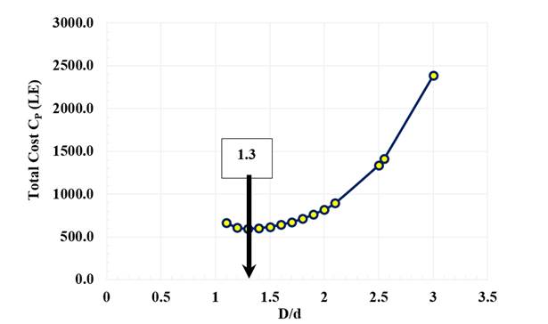
For this purpose, the total pipe cost C_P is computed at different pipe-nozzle diameter ratios D/d. The results are shown in Table 2, which is also used to plot C_P versus D/d as shown in Figure 3. Investigation of both table and figure show the following: (A) Diameter ratios D/d above 1.6 give high pipe costs, while smaller D/d give low total costs. (B) The minimum pipe cost lies at D/d = 1.4, which is also reached by the solution of the derived Equation 10. This assures the rigidity of the derived solution for computing pipe-nozzle diameter ratio D/d.

Figure 2

                                                                      

Figure 2 Graphical Solution of Equation 10 Based on Minimum Pipe Cost for the Illustrative Example

 

Table 2

Table 2 Results for Total Pipe Cost CP Versus Diameter Ratio D/d for the Illustrative Example
D/d	C	Cv	K	CP (LE)
1.1	0.8991	0.5062	2.9027	666.9
1.2	0.8919	0.6418	1.4279	606.6
1.3	0.8854	0.7137	0.9630	596.7
1.4	0.8794	0.7563	0.7483	602.6
1.5	0.8738	0.7827	0.6321	617.8
1.6	0.8686	0.7996	0.5640	641.0
1.7	0.8638	0.8104	0.5226	672.3
1.8	0.8593	0.8173	0.4970	712.2
1.9	0.8550	0.8215	0.4817	761.8
2	0.8510	0.8239	0.4730	822.2
2.1	0.8472	0.8251	0.4689	894.8
2.5	0.8337	0.8229	0.4766	1339.4
2.55	0.8322	0.8223	0.4791	1416.0
3	0.8198	0.8147	0.5065	2388.1

 

3. RESULTS AND DISCUSSIONS

3.1. Evaluation of minimum cost

3.1.1.  Variation of C_P versus D/d (variable pipe cost coefficient a)

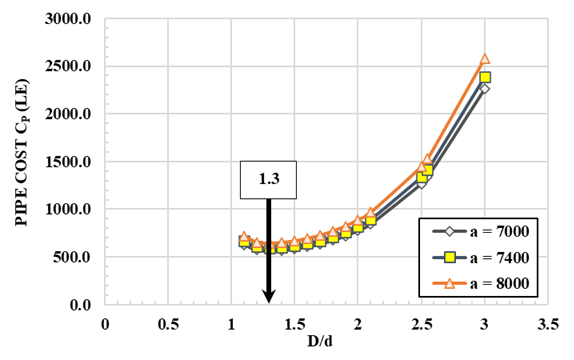
The data given within the illustrative example are x = 2.5, F = 0.05, and L/D = 200, while the pipe cost factor a is taken 7000, 7400, and 8000, Table 3. The corresponding plots of C_P versus D/d at various pipe cost factor (a) are shown in Figure 4. Investigation of these plots shows the following:

1)     The plots exhibit similar trends.

2)     The increase of diameter ratio D/d leads to increase of C_P, and the rate of increase being at higher D/d (1.8-3), Figure 4.

3)     At a fixed value of D/d, C_P increases with increase of the pipe cost coefficient a.

4)     All the plots indicate that the minimum pipe cost C_P takes place at a unique diameter ratio of 1.3, Table 3.

 Figure 3

                                                                    

Figure 3 Plot of Total Pipe Cost CP Versus Diameter Ratio D/d for the Illustrative Example

 

 

 

Figure 4

                                                                     

Figure 4 Plots of CP Versus D/d for the Illustrative Example at Various Pipe Cost Exponent A

 

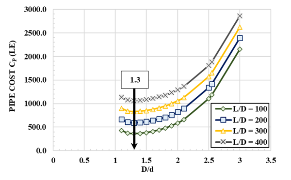
3.1.2.  Variation of C_P versus D/d (variable relative distance L/D)

The data given within the illustrative example are:

x = 2.5, F = 0.05, a = 7400, and L/D = (100, 200, 300, and 400), Table 4. The corresponding plots are shown in Figure 5. Investigation of these plots leads to the following: (A) The plots exhibit similar trends. (B) The pipe cost C_P increases with increase of D/d, the rate of increase being higher at larger D/d ratios (1.8-3.0), Figure 5. (C) In all the plots, it is found that, at a particular value of D/d, C_P increases with increase of e/D, which is logical. (D) In all the plots, the minimum C_P is at D/d = 1.3, Table 4.

Table 3

Table 3 Results of Total Pipe Cost CP Versus Diameter Ratio D/D For Various Unit Pipe Exponent A
D/d	C	Cv	K		CP (LE)
					a
				7000	7400	8000
1.1	2.9027	0.5062	2.9027	630.9	666.9	721.0
1.2	0.8919	0.6418	1.4279	573.8	606.6	655.8
1.3	0.8854	0.7137	0.9630	564.5	596.7	645.1
1.4	0.8794	0.7563	0.7483	570.0	602.6	651.4
1.5	0.8738	0.7827	0.6321	584.4	617.8	667.9
1.6	0.8686	0.7996	0.5640	606.4	641.0	693.0
1.7	0.8638	0.8104	0.5226	635.9	672.3	726.8
1.8	0.8593	0.8173	0.4970	673.7	712.2	770.0
1.9	0.8550	0.8215	0.4817	720.6	761.8	823.6
2	0.8510	0.8239	0.4730	777.8	822.2	888.9
2.1	0.8472	0.8251	0.4689	846.5	894.8	967.4
2.5	0.8337	0.8229	0.4766	1267.0	1339.4	1448.0
2.55	0.8322	0.8223	0.4791	1339.5	1416.0	1530.8
3	0.8198	0.8147	0.5065	2259.1	2388.1	2581.8

 

3.1.3.  Variation of C_P versus D/d (variable e/D and F)

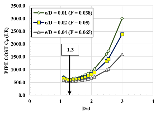
The data given within the illustrative example are x = 2.5, a = 7400, and L/D = 200, The variable is e/D (0.01, 0.02, 0.04) which corresponds to F (0.038, 0.05, 0.065), Table 5. The corresponding plots are shown in Figure 6. Investigation of these plots lead to the following conclusions:

(A) All the plots exhibit similar trends. (B) In each plot, C_P increases with increase of D/d being from (1.8 to 3.0). (C) In the plots, at a particular value of D/d, C_P decreases with increase of relative roughness e/D, the rate of decrease being larger for higher D/d (2.0 to 3.0). (D) In all the plots, the minimum cost C_P occurs at D/d = 1.3. This is attributed to that, in each case solving of Equation 10 for the minimum cost diameter ratio D/d, the left-hand side of the equation converges to D/d = 1.3.

Table 4

Table 4 Results of Total Pipe Cost CP Versus Diameter Ratio D/D for Various Relative Length
D/d	C	Cv	K		CP (LE)
				L/D
				100	200	300	400
1.1	0.8991	0.5062	2.9027	432.9	666.9	900.9	1134.9
1.2	0.8919	0.6418	1.4279	372.6	606.6	840.6	1074.6
1.3	0.8854	0.7137	0.9630	362.7	596.7	830.8	1064.8
1.4	0.8794	0.7563	0.7483	368.6	602.6	836.6	1070.6
1.5	0.8738	0.7827	0.6321	383.8	617.8	851.8	1085.8
1.6	0.8686	0.7996	0.5640	407.0	641.0	875.0	1109.0
1.7	0.8638	0.8104	0.5226	438.3	672.3	906.3	1140.3
1.8	0.8593	0.8173	0.4970	478.2	712.2	946.2	1180.2
1.9	0.8550	0.8215	0.4817	527.8	761.8	995.8	1229.8
2	0.8510	0.8239	0.4730	588.2	822.2	1056.2	1290.2
2.1	0.8472	0.8251	0.4689	660.8	894.8	1128.8	1362.9
2.5	0.8337	0.8229	0.4766	1105.4	1339.4	1573.4	1807.4
2.55	0.8322	0.8223	0.4791	1182.0	1416.0	1650.0	1884.0
3	0.8198	0.8147	0.5065	2154.1	2388.1	2622.2	2856.2

 

 

 

 

 

 

 

Figure 5

                                                                     

Figure 5 Plots of CP Versus D/D for the Illustrative Example at Various Relative Distance L/D

 

  Figure 6

                                                                     

Figure 6 Plots of CP versus D/d for the Illustrative Example at Various Relative Roughness e/D

 

3.1.4.  Variation of C_P versus D/d (variable e/D and F)

The data given within the illustrative example are x = 2.5, a = 7400, and L/D = 200, The variable is e/D (0.01, 0.02, 0.04) which corresponds to F (0.038, 0.05, 0.065), Table 5. The corresponding plots are shown in Figure 6. Investigation of these plots lead to the following conclusions:

(A) All the plots exhibit similar trends. (B) In each plot, C_P increases with increase of D/d being from (1.8 to 3.0). (C) In the plots, at a particular value of D/d, C_P decreases with increase of relative roughness e/D, the rate of decrease being larger for higher D/d (2.0 to 3.0). (D) In all the plots, the minimum cost C_P occurs at D/d = 1.3. This is attributed to that, in each case solving of Equation 10 for the minimum cost diameter ratio D/d, the left-hand side of the equation converges to D/d = 1.3.

Table 5

Table 5 Results of CP versus D/d for various L/D (100, 200, 300, and 400) and e/D (0.01, 0.02, and 0.04)
D/d	C	Cv	K	CP (LE)
				e/D
				0.01	0.02	0.04
1.1	0.8991	0.5062	2.9027	729.7	666.9	585.0
1.2	0.8919	0.6418	1.4279	650.4	606.6	549.5
1.3	0.8854	0.7137	0.9630	637.4	596.7	543.7
1.4	0.8794	0.7563	0.7483	645.0	602.6	547.2
1.5	0.8738	0.7827	0.6321	665.1	617.8	556.1
1.6	0.8686	0.7996	0.5640	695.7	641.0	569.8
1.7	0.8638	0.8104	0.5226	736.8	672.3	588.2
1.8	0.8593	0.8173	0.4970	789.3	712.2	611.7
1.9	0.8550	0.8215	0.4817	854.6	761.8	640.8
2	0.8510	0.8239	0.4730	934.1	822.2	676.4
2.1	0.8472	0.8251	0.4689	1029.6	894.8	719.1
2.5	0.8337	0.8229	0.4766	1614.5	1339.4	980.6
2.55	0.8322	0.8223	0.4791	1715.4	1416.0	1025.7
3	0.8198	0.8147	0.5065	2994.5	2388.1	1597.5

 

Table 6

Table 6 Results of D/d, PJ and CP using Equation 10 and the Conventional Formula       (F=0.05 and L/D (100-400) for the illustrated example)
L/D	Eq. (10)			Conventional Formula
	D/d	PJ	CP	D/d	PJ	CP
		(KW)	(LE)		(KW)	(LE)
100	1.3	0.4	303.8	1.78	1.16	336.1
200	1.3	0.79	607.5	2.115	1.1	951.9
300	1.3	1.124	911.3	2.34	1.02	1846.7
400	1.3	1.575	926.6	2.5	0.92	3070.4

 

3.2. Comparison between minimum cost and conventional formulae computing D/d

For this purpose, Table 6 is constructed showing the important parameters to be compared using both formulae, where C_P is calculated at F = 0.05, and L/D as taken (100, 200, 300, and 400).

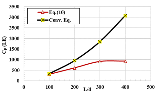
Investigation of Table 6 indicates that: (A) The derived Equation 10 shows a unique value for D/d = 1.3 which satisfies the minimum C_P, while in the conventional formula, D/d increases with L/D. (B) Eq. (10), shows that P_J increases with increase of L/D and vice versa by the conventional formula, Figure 7. According to Equation 10, the increase in the jet power ranges from 14.5 to 55.6 percent by increase of L/D, while in the conventional formula shows a decrease in jet power by 26 percent. (C) With respect to the pipe cost C_P, Table 6 and Figure 6 and Figure 8, in both equations, C_P increases with increase of e/D, but Equation 10 shows marked reduction in C_P with increase of L/D. Also, Equation 10 achieves lower values of C_P compared with the conventional formula for example, at L/D = 100, the conventional formula, shows an increase of C_P of 10.6 percent and 231.4 percent at L/D = 400, indicating that Equation 10, is more reliable than the conventional one.

  Table 7

Table 7 Results of D/d, PJ and CP using Equation 10 and the Conventional Formula       (L/D=200, for the Illustrative Example)
e/D	Eq. (10)			Conventional Formula
	D/d	PJ	CP	D/d	PJ	CP
		(KW)	(LE)		(KW)	(LE)
0.01	1.4	1	651.7	1.98	1.28	957.8
0.02	1.4	0.79	607.5	2.115	1.1	951.9
0.04	1.4	0.62	575.5	2.252	0.84	954.8

 

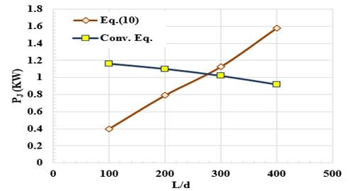
Figure 7

                                                                     

Figure 7 Results of D/d Versus PJ using Equation 10 and Conventional Formula for L/D=200

 

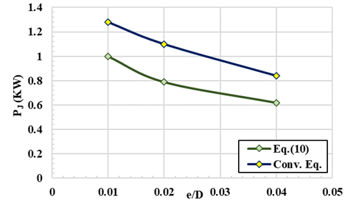
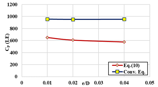
On the other hand, Table 7 is constructed for D/d, P_J, and C_P using Equation 10 and the conventional formula at L/D = 200, e/D (0.01, 0.02, and 0.04) or F (0.038, 0.05, and 0.065) respectively. Table 7 and the plots in Figure 9, indicate the following: (A) The two plots of PJ versus e/D, have the same trend, indicating that P_J decreases with increase of e/D, due to the frictional effects in the approach pipe, but the conventional equation gives higher values of PJ, Figure 9, this is attributed to the nature of this equation. (B) With respect to the plots of C_P and e/D both equations, have similar trends with a marked reduction of C_P indicated by    Equation 10, Figure 10 Plots of C_P Versus e/D for the Illustrative Example at L/D=200. However, the use of Equation 10 shows, reduction in C_P ranges from 34 at e/D=0.01 and 39.7 % at e/D=0.04, which indicates the validity of Equation 10 and that the conventional formula is approximate.

Figure 8

                                                                       

Figure 8 Results of D/d Versus CP using  Equation 10 and Conventional Formula for L/D=200

 

Figure 9

                                                                     

Figure 9 Plots of PJ Versus e/D for the Illustrative Example at L/D=200

 

Figure 10

                                                                     

Figure 10 Plots of CP Versus e/D for the Illustrative Example at L/D=200

 

Finally, it may be stated that, the results obtained for computing the minimum cost of pipe-nozzle diameter ratio in discharge lines delivering free jets, by the derived Equation 10, indicate the validity of the equation in estimating the economic pipe-nozzle diameter ratio, D/d, the corresponding power of the jet P_J, and the minimum cost of the discharge line C_P.

 

4. CONCLUSIONS and RECOMMENDATIONS

The following conclusions can be reached as follows:

1)     Equation 10, derived for computing the economic nozzle-pipe diameter ratio D/d in discharge lines delivering free jets, is applicable over practical ranges of relative distance L/D and relative roughness e/D under rough, turbulent flow conditions (in approach pipe). For the time being, L/D ranges from 50 to 500, e/D ranges from 0.01 to 0.05, and Rn from 105 to 106.

2)     In the given illustrated example, Equation 10derived for D/d ratio, is solved by trial and error, and shows that the economic diameter ratio is close to 1.3, where the total pipe cost has a minimum value. Also, the results of C_P, show that the derived equation holds good for D/d ratios from 1.1 to 3.0, Table 5, and could be applied without the need for a computer program.

3)     Investigation of Equation 10, shows that the economic diameter ratio D/d depends on; the relative distance L/D, the coefficient of friction F in the approach pipe, the minor loss coefficient of the nozzle K, and the pipe cost exponent x.

4)     On comparison basis between Equation 10 and the conventional formula, at (F = 0.05, L/D = 200), the first shows that at the economic ratio D/d = 1.3, the pipe cost C_P = 607.5LE and the power of the jet, P_J = 0.97KW, while in the conventional equation, D/d = 2.115, C_P = 951.9LE and the power of the jet, P_J = 1.1KW. However, the derived Equation 10, realizes a reduction in C_P by 56.7% and in P_J by 39.2%. But the reduction in C_P is wanted as it is the main purpose of the present study.

5)     On the other hand, at F = 0.05 and by increase of L/D to 400, still economic D/d = 1.4, P_J = 1.575KW, and C_P = 9266LE by the use of the derived Eq. (10). While the conventional formula shows that D/d = 2.5, PJ = 0.92KW, and C_P = 30704LE, Table 6. However, at F = 0.05 and L/D = 400, it is found that Equation 10 attains a reduction in C_P by 231% with an increase in P_J by 41.6% compared with the conventional formula.

6)     Considering the friction in the approach pipe, it has the effect of decreasing P_J when computed by the conventional formula. While use of Equation 10, shows reduction in C_P ranging from 34 to 39.7 %, indicating the validity of the derived equation.

7)     It may be stated that, the evaluation study of Equation 10 reflects the rigidity and reliability of this equation in computing the economic pipe-nozzle diameter ratio D/d in discharge lines delivering free jets and for the time being, good results are obtained at F = 0.05 and L/D = 400, higher PJ and lower C_P.

 

 

 

 

5. NOMENCLATURE

F = Coefficient of friction in the approach pipe,

D = Mean diameter of approach pipe,

L_e = Equivalent length of approach pipe,

g = Gravitational acceleration,

V_p = Mean velocity of water in the approach pipe,

D/d = Pipe-nozzle diameter ratio

V_J = Absolute velocity of the jet at the nozzle opening,

d = diameter of the nozzle opening.

K = Minor loss coefficient of the nozzle,

L = Length of approach pipe,

C_P = Pipe Cost,

C_v = Coefficient of velocity of the nozzle,

a = pipe cost function,

x = Pipe cost exponent,

C = Flow coefficient of the nozzle,

L/D = Relative distance,

P_J = power of the jet,

e = Roughness height in approach pipe,

e/D = Relative roughness of pipe,

P_J = Power of the jet.

 

CONFLICT OF INTERESTS

None. 

 

ACKNOWLEDGMENTS

None.

 

REFERENCES

BETE for Nozzle Performance Engineering (2022). Spray Nozzles For The Waste Management Industry.

De Cock, N. (2017). Design of a Hydraulic Nozzle with a Narrow Droplet Size Distribution. Phd Dissertation, Université De Liège, Liège, Belgium.

Featherstone, R. E., and El-Jumaily, K. K. (1983). Optimal Diameter Selection for Pipe Networks. Journal of Hydraulic Engineering, 109(2), 221-234, Computer-Aided Design, 15(5), 300. https://doi.org/10.1061/(ASCE)0733-9429(1983)109:2(221).

Joseph B. Franzini, E., and Finnemore, J. (2010). Fluid Mechanics with Engineering Applications. Mcgraw-Hill College, MA, USA, 10th International Edition.

Koirala, R., Ve, Q. L., Zhu, B., Inthavong, K., and Date, A. (2021). A Review on Process and Practices in Operation and Design Modification of Ejectors. Fluids, 6(11), 409. https://doi.org/10.3390/fluids6110409.

Mazzoleni, A. P. (1994). Design of High-Pressure Waterjet Nozzles. Alabama Univ., Research Reports : 1994 NASA (ASEE Summer Faculty Fellowship Program).

Medan, N., Banica, M., and Ravai-Nagy, S. (2017). Full Factorial DOE to Determine and Optimize the Equation of Impact Forces Produced by Water Jet Used in Sewer Cleaning. MATEC Web of Conferences, 137, 07003.  https://doi.org/10.1051/matecconf/201713707003.

Poeck, E. C. (2008). Performance Evaluation of Various Nozzle Designs for Waterjet Scaling in Underground Excavations, Phd Dissertation, Colorado School of Mines.

Radkevich, M., Abdukodirova, M., Shipilova, K., and Abdullaev, B. (2021). Determination of the Optimal Parameters of the Jet Aeration. IOP Conference Series: Earth and Environmental Science, 939(1), 012029.

Renjie, L., Xiaochen, L., Jin-Shi, L., and Zhang, X. (2020). Design and Simulation of Curved Nozzle for Removing the Fish Scale by the Water Jet. U.P.B. Science Bulletin, Series D, 82(1).

Schwartzentruber, J., Narayanan, C., Papini, M., and Liu, H. T. (2016). Optimized Abrasive Waterjet Nozzle Design Using Genetic Algorithms. The 23rd International Conference on Water Jetting, Seattle, USA.

Sharp, B. B. (1985). Economics of Pumping and the Utilization Factor. Journal of Hydraulic Engineering, 111(11), 1386–1395. https://doi.org/10.1061/(ASCE)0733-9429(1985)111:11(1386).

Simon, A.L.SS.  (1987). Hydraulics. John Wiley and Sons Ltd, 3rd Edition.

Somaida M., El-Zahar M., and Sharaan M. (2012). The Use of Computer Simulation and Analytical Solutions for Optimal Design of Pipe Networks Supplied from a Pumped-Groundwater Source. Port Said Engineering Research Journal, 16(1), 106-117.

Somaida, M. M. (1994). Optimal Design of Pipe-Nozzle Lines Discharging Free Jets. Port Said Engineering Research Journal, 6(1).

Somaida, M. M., El-Zahar, M. M., Hamed, Y. A., and Sharaan, M. S. (2013). Optimizing Pumping Rate in Pipe Networks Supplied by Groundwater Sources. KSCE Journal of Civil Engineering, 17(5), 1179-1187. https://doi.org/10.1007/s12205-013-0116-4.

Somaida, M., Elzahar, M., and Sharaan, M. (2011). A Suggestion of Optimization Process for Water Pipe Networks Design. International Conference on Environment and Bio-Science IPCBEE, 21, 68-73.

Streeter, V. L., Wylie, E. B. (1985). Fluid Mechanics. Mcgraw-Hill Education, 8th Edition.

Swaffield, J., Jack, L., Douglas, J. F. and John Gasiorek. (2011). Fluid Mechanics, Pearson Canada, 6th Edition.

Wright, D., Wolgamott, J., and Zink, G. (2003). Water Jet Nozzle Material Types. WJTA American Waterjet Conference, 17-19.