
|
|
|
|
PENETRATIVE THERMO-GRAVITATIONAL AND SURFACE- TENSION DRIVEN CONVECTION IN A FERROFLUID LAYER THROUGH VOLUMETRIC INTERNAL HEATING WITH VARIABLE VISCOSITYMahesh Kumar R 1 1 Department of Mathematics, M E S Pre-University College of Arts, Commerce and Science, Bengaluru- 560003, India2 Department of Mathematics, Dr. Ambedkar Institute of Technology, Bangalore, India |
|
||
|
|
|||
|
Received 20 March 2022 Accepted 02 April 2022 Published 27 April 2022 Corresponding Author Mahesh Kumar R, rmaheshkumar78@rediffmail.com DOI 10.29121/ijetmr.v9.i4.2022.1140 Funding: This research
received no specific grant from any funding agency in the public, commercial,
or not-for-profit sectors. Copyright: © 2022 The
Author(s). This is an open access article distributed under the terms of the
Creative Commons Attribution License, which permits unrestricted use, distribution,
and reproduction in any medium, provided the original author and source are
credited.
|
ABSTRACT |
|
|
|
This work pertaining to analytical and numerical
studies on FTC in a FF layer with impact of coupled buoyancy-gravitational
and surface-tension forces through the strength of internal heat source on
the system subjected to the magnetic field dependent (MFD) viscosity effect.
The lower boundary is considered to be rigid at either conducting or
insulating to temperature perturbations, while upper boundary free open to
the atmosphere is flat and subject to a Robin-type of thermal boundary
condition. The Rayleigh-Ritz method with Chebyshev polynomials of the second
kind as trial functions is employed to extract the critical stability
parameters numerically. The onset of FTC is delayed with an increase in MFD (d ) parameter and Biot number (Bi) but opposite is the case with an increase in Rayleigh
number (M1), non-linearity of fluid magnetization (M3) and
strength of internal heat source (Ns). Their effects are complementary in the
sense that the critical Mac and Rmc decrease with an
increase in Rt. |
|
||
|
Keywords: Buoyancy-Gravitational, Surface-Tension
Forces, Galerkin Technique, Ferrofluids, Volumetric Internal Heating, MFD
Viscosity 1. INTRODUCTION
Ferrofluids (FFs) are synthesized by suspending single domain
ferromagnetic nanoparticles stabilized in various nonmagnetic carrier fluids,
which exhibit both magnetic and fluid properties Rosensweig
(1985), Shliomis
(1974). These fluids are now termed as magnetic nanofluids
and the study of such fluids has been a subject of intensive investigations
over decades due to their potential applications in magnetically heat
controlled thermosiphons for technological purposes Charles
(2002), Blums
(2002). Thermal convection in an FF layer in the
occurrence of magnetic field, called ferro- thermal-convection (FTC), has
been studied extensively both theoretically and experimentally over the years
to understand the heat transfer systems and the details are sufficiently
documented in the review article by Nkurikiyimfura
et al. (2013).
Most FFs are either water based, or oil based. The viscosity of water
is far more sensitive to temperature variations and oils are known to have
viscosity decreasing exponentially with temperature rather than linearly.
Realizing the importance, several investigators considered exponential
variation in |
|
||


viscosity with temperature in analysing thermal convective instability in horizontal fluid layers, but the studies were limited to ordinary viscous fluids Kassoy and Zebib (1975), Blythe and Simpkins (1981), Patil and Vaidyanathan (1981), Patil and Vaidyanathan (1982). To our knowledge, no attention has been given to convective instability problems involving FFs, despite the importance of FFs in many heat transfer applications. For example, in a rotating shaft seal involving FFs the temperature may rise above 1000C at high shaft surface speeds. A similar situation may arise in the use of FFs in loudspeakers Lebon and Cloot (1986). The onset of FTC in a horizontal FF layer with temperature dependent viscosity in exponentially is examined Shivakumara et al. (2012).
In many natural phenomena, the study of penetrative FTC in a saturated porous layer Nanjundappa et al. (2011) with the internal heating source and applied Brinkman extended Darcy model in the momentum equation analyzed the internal heat generation effect on the onset of FTC in an FF saturated porous layer Nanjundappa et al. (2011), Nanjundappa et al. (2012). Savitha et al. (2021) investigated the penetrative FTC in an FF-saturated high porosity anisotropic porous layer via uniform internal heating. Thus, the purpose of the present chapter is to study a general problem of coupled thermo- gravitational and surface-tension FC in an FF layer with magnetic field dependent (MFD) viscosity. The study helps to understanding the control of FTC by MFD viscosity, which is constructive in various problems associated by heat transfer particularly in material-science processing. In the current study, the bottom surface is rigid with either constant temperature or uniform heat flux, while the upper is un-deformable free surface of surface tension forces. Besides, the Neumann-type of boundary condition is imposed on the upper surface. Several investigators have studied both types of instabilities in isolation or together in a horizontal FF layer.
2.
PROBLEM
FORMULATION
Consider a layer of horizontal Boussinesq FF of
constant depth ![]() with a uniformly volumetric heat source strength,
with a uniformly volumetric heat source strength, ![]() , and in the
occurrence of perpendicular magnetic field
, and in the
occurrence of perpendicular magnetic field ![]() . The surfaces are maintained the constant temperatures at
. The surfaces are maintained the constant temperatures at ![]() and
and ![]() . The gravity,
. The gravity, ![]() , acting downward direction, where
, acting downward direction, where ![]() is the z-direction of unit vector. The stream of Bénard-Marangoni
convection for thermocapillary force,
is the z-direction of unit vector. The stream of Bénard-Marangoni
convection for thermocapillary force, ![]() (surface tension force), is given by
(surface tension force), is given by
![]() Equation 1
Equation 1
where sT, s0 are positive constants.
The Maxwell’s equations for magnetic field are implemented by
![]() or
or ![]() Equation 2
Equation 2
![]() Equation 3
Equation 3
were
![]() Equation
4
Equation
4
With
![]() Equation 5
Equation 5
and
![]() Equation 6
Equation 6
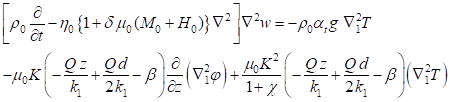
The equation of momentum with variable viscosity is
![]() Equation 7
Equation 7
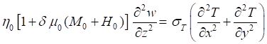
The heat equation with internal heating
Q
is
![]() Equation 8
Equation 8
The conservation of mass equation
is
![]() Equation 9
Equation 9
The state equation is
![]() Equation
10
Equation
10
Here ![]() is the velocity, p is the pressure, t is the time,
is the velocity, p is the pressure, t is the time, ![]() is the magnetic
induction and
is the magnetic
induction and ![]() is the intensity of
magnetic field,
is the intensity of
magnetic field, ![]() is the magnetization,
is the magnetization, ![]() is the magnetic
permeability of vacuum, CV,H
is the specific heat capacity at constant volume and magnetic field per unit
mass, and kt is the thermal conductivity,
is the magnetic
permeability of vacuum, CV,H
is the specific heat capacity at constant volume and magnetic field per unit
mass, and kt is the thermal conductivity, ![]() is the magnetic
susceptibility and
is the magnetic
susceptibility and ![]() is the pyromagnetic co-efficient,
is the pyromagnetic co-efficient, ![]() is the thermal
expansion coefficient,
is the thermal
expansion coefficient, ![]() is the density at
is the density at ![]() ,
, ![]() ,
, ![]() ,
, ![]() and the last term of Equation
7 denotes as
and the last term of Equation
7 denotes as ![]() is the rate of strain
tensor. The fluid is assumed to be incompressible having variable viscosity.
Experimentally, it has been demonstrated that the magnetic viscosity has got
exponential variation, with respect to magnetic field Rosenwieg
et al. (1969) As a first
approximation, for small field variation, linear variation of magnetic
viscosity has been used in the form
is the rate of strain
tensor. The fluid is assumed to be incompressible having variable viscosity.
Experimentally, it has been demonstrated that the magnetic viscosity has got
exponential variation, with respect to magnetic field Rosenwieg
et al. (1969) As a first
approximation, for small field variation, linear variation of magnetic
viscosity has been used in the form ![]() , where
, where ![]() is the variation
coefficient of magnetic field dependent viscosity and is considered to be
isotropic Vaidyanathan et al. (2002),
is the variation
coefficient of magnetic field dependent viscosity and is considered to be
isotropic Vaidyanathan et al. (2002), ![]() is taken as viscosity
of the fluid when the applied magnetic field is absent.
is taken as viscosity
of the fluid when the applied magnetic field is absent.
The undisturbed quiescent state
![]() Equation 11
Equation 11
![]() Equation 12
Equation 12
![]() Equation
13
Equation
13
![]() Equation 14
Equation 14
![]() Equation
15
Equation
15
Here we note that, ![]() ,
, ![]() ,
, ![]() are distributed
parabolically with the height of the FF layer due to the existence of
volumetric heat source,
are distributed
parabolically with the height of the FF layer due to the existence of
volumetric heat source, ![]() . However, for
. However, for ![]() , the distributions
of basic state are linear in z.
, the distributions
of basic state are linear in z.
To study the stability of the quiescent state and perturb the relevant variables in the corresponding governing equations with framework of the linear theory
![]() ,
, ![]() , T =
, T = ![]() ,
, ![]() ,
, ![]() Equation 16
Equation 16
Let the components of ![]()
![]()
be perturbed the magnetization and magnetic field, respectively.
Using these in Equation 2,Equation 6, linearizing, we obtain
![]() Equation 17
Equation 17
![]() Equation 18
Equation 18
![]() Equation 19
Equation 19
From Equation 17,Equation 19 and it is considered
that ![]() ;
; ![]() .
.
Experimentally, Rosenwieg
et al. (1969) has demonstrated the
exponential variation in magneto-viscosity, ![]() , where
, where ![]() is the variation of
viscosity coefficient. Since the first approximation of small (linear) field
variation in magneto-viscosity has been used. Substituting Equation 16 in Equation
7
and applying the basic state solutions, removing the pressure p by
operating two times of curl on the resulting equations and linearizing together
with
is the variation of
viscosity coefficient. Since the first approximation of small (linear) field
variation in magneto-viscosity has been used. Substituting Equation 16 in Equation
7
and applying the basic state solutions, removing the pressure p by
operating two times of curl on the resulting equations and linearizing together
with ![]() , then gives
, then gives
 Equation 20
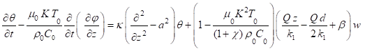
As before, using
Equation 16 ,Equation 8 and applying basic state solutions, and linearizing, we
obtain
![]() Equation 21
Equation 21
Where ![]()
Finally, Equation 2,Equation 3, after using Equation 16 together with Equation 17,Equation 19, yields (after neglecting
primes)
![]() Equation 22
Equation 22
As the customary of convective instability analysis for
each variable of ![]() is expanded in
following form by assuming the normal mode hypothesis (separation of variables)
is expanded in
following form by assuming the normal mode hypothesis (separation of variables)
![]() Equation
23
Equation
23
Substituting into Equation 20,Equation 22, we get
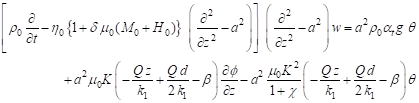 Equation 24
 Equation 25
![]() Equation 26
Equation 26
Thus, Equation 24,Equation 26 are the governing linearized perturbation equations and they are non- dimensional zed using the following quantities:
![]()
![]()
![]() Equation
27
Equation
27
After using Equation 25 in Equation 22, Equation 24, we obtain (ignoring the asterisks)
![]()
![]() Equation 28
Equation 28
![]() Equation 29
Equation 29
Where ![]() .
.
We set
![]() Equation 30
Equation 30
Here, ![]() denoted as the growth
rate, which is complex frequency.
denoted as the growth
rate, which is complex frequency.
Substituting into Equation 26 ,Equation 28, we obtain
![]() Equation 31
Equation 31
![]() Equation 32
Equation 32
![]() Equation 33
Equation 33
The boundary conditions for these equations are
1. Lower boundary rigid-ferromagnetic at fixed temperature as
![]()
2. Lower boundary rigid-ferromagnetic at fixed heat flux as
![]() Equation 34
Equation 34
After linearizing the equations for balancing the surface tension gradient with shear stress at the free surfaces (Pearson 1958), we have
![]() ;
; ![]() Equation 35
Equation 35
where ![]() is the surface tension
and
is the surface tension
and ![]() ,
, ![]() are the shear stress Using Equation 37
yields
are the shear stress Using Equation 37
yields
![]() Equation 36
Equation 36
For most of the liquids as the temperature rises, the variation between the liquid and its vapor phase decreases. Thus, the suitable boundary conditions of surface tension at the free surfaces are
![]() ;
; Equation 37
Using Equation 39 and non-dimensionlizing the equations, we get
![]() and
and ![]() Equation 38
Equation 38
where, ![]() denoted as the
Marangoni number
denoted as the
Marangoni number ![]() .
.
Upper boundary free ferromagnetic at fixed heat flux is
![]() Equation 39
Equation 39
were, Bi denoted as the Biot number ![]()
3. METHOD OF SOLUTION
The GT is applied to obtain the problem of eigenvalue
is to study the linear system of Equation 32 with Equation 35 and Equation 41.
The unknown factors ![]() can be expanded upon
the complete set:
can be expanded upon
the complete set:
![]() Equation
40
Equation
40
Substitute in Equation 32 Equation 32, multiplying the
resulting equations respectively by ![]() ,
, ![]() ,
, ![]() and carrying out the integration by parts from z = 0 to z = 1
and using Equation 35 and Equation 41 we obtain
and carrying out the integration by parts from z = 0 to z = 1
and using Equation 35 and Equation 41 we obtain
![]() Equation
41
Equation
41
![]() Equation 42
Equation 42
![]() Equation 43
Equation 43
From Equation 43,Equation 45 have a non-trivial solution if
 Equation 44
Were
![]()
![]()
![]() ,
, ![]()
![]()
![]() ,
, ![]()
Where ![]()
The eigenvalue is extracted from Equation 45. A trivial function ![]()
![]() ,
, ![]() can be considered to
satisfy the boundary conditions Equation 35, Equation 36 and Equation 41
by selecting the trial functions as
can be considered to
satisfy the boundary conditions Equation 35, Equation 36 and Equation 41
by selecting the trial functions as
![]() ,
, ![]()
(i) For lower insulating case: ![]() , Equation 45
, Equation 45
(ii) For lower
conducting case: ![]()
Here![]() s denoted as the second kind Tchebyshev’ polynomials, such
that
s denoted as the second kind Tchebyshev’ polynomials, such
that ![]()
![]() satisfy Equation 35, Equation 36 and Equation 41 except, namely
satisfy Equation 35, Equation 36 and Equation 41 except, namely ![]() and
and ![]() however the residual
from this equations is incorporated as a residual from Eqs. Equation 32,Equation 34
however the residual
from this equations is incorporated as a residual from Eqs. Equation 32,Equation 34
4. NUMERICAL RESULTS AND DISCUSSION
It may be illustrated that Equation
41 with w = 0 leads to the Marangoni
number ![]() corresponding wavenumber a with
corresponding wavenumber a with ![]() and
and ![]() . The inner products concerned in the equations are assessed
analytically in order to keep away from the errors in numerical integration.
The reveals the computations that the convergence in resulting Mac
crucially depends on
. The inner products concerned in the equations are assessed
analytically in order to keep away from the errors in numerical integration.
The reveals the computations that the convergence in resulting Mac
crucially depends on ![]() . The presented results for i = j = 8
the order at which the convergence is attained, in general. The critical Marangoni number
. The presented results for i = j = 8
the order at which the convergence is attained, in general. The critical Marangoni number ![]() is determined by
corresponding critical wavenumber
is determined by
corresponding critical wavenumber ![]() . The results thus attained for different
. The results thus attained for different ![]() and
and ![]() are existing graphically in
Figure 2 and also in Table 1 and Table 2
are existing graphically in
Figure 2 and also in Table 1 and Table 2
To solve the eigenvalue problem from Equation 41 by employing the Galerkin-type of WRM. In order to confirm the
numerical technique is applied, the values ![]() and
and ![]() are very close to the existing values of Nield (1964) for
are very close to the existing values of Nield (1964) for ![]() and Sparrow
et al. (1964) for
and Sparrow
et al. (1964) for ![]() under the limiting condition in Table 1 and Table 2, respectively. The comparisons of calculated present results
agree well with results of previous numerical investigations are given in Table 1 and Table 2. It is evident that
the results are in good agreement between the present and published previously.
This validates the applicability and exactness of the method applied in solving
the convective instability problem considered
under the limiting condition in Table 1 and Table 2, respectively. The comparisons of calculated present results
agree well with results of previous numerical investigations are given in Table 1 and Table 2. It is evident that
the results are in good agreement between the present and published previously.
This validates the applicability and exactness of the method applied in solving
the convective instability problem considered
|
Table 1 Comparison of (Mac, ac) and (Rtc, ac) for
Rm =d=0 |
||||||||
|
Nield
[18] |
Present
analysis |
|||||||
|
Lower
insulating |
Lower
conducting |
Lower
insulating |
Lower
Conducting |
|||||
|
Bi |
Mac |
ac |
Rc |
ac |
Mac |
ac |
Rc |
ac |
|
0 |
79.607 |
1.993 |
669 |
2.086 |
79.6067 |
1.9929 |
668.998 |
2.0856 |
|
0.01 |
79.991 |
1.997 |
670.38 |
2.089 |
79.9913 |
1.9966 |
670.381 |
2.0888 |
|
0.1 |
83.427 |
2.028 |
682.36 |
2.117 |
83.4267 |
2.0281 |
682.36 |
2.1162 |
|
0.2 |
87.195 |
2.06 |
694.78 |
2.144 |
87.1951 |
2.0603 |
694.779 |
2.1437 |
|
0.5 |
98.256 |
2.142 |
727.42 |
2.212 |
98.2562 |
2.1423 |
727.422 |
2.2116 |
|
1 |
116.127 |
2.246 |
770.57 |
2.293 |
116.127 |
2.2462 |
770.57 |
2.2928 |
|
2 |
150.679 |
2.386 |
831.27 |
2.393 |
150.679 |
2.3864 |
831.27 |
2.3926 |
|
5 |
250.598 |
2.598 |
925.51 |
2.519 |
250.598 |
2.5978 |
925.51 |
2.519 |
|
10 |
413.44 |
2.743 |
989.49 |
2.589 |
413.44 |
2.7426 |
989.492 |
2.5889 |
|
20 |
736 |
2.852 |
1036.3 |
2.632 |
736 |
2.8524 |
1036.3 |
2.6323 |
|
50 |
1699.62 |
2.941 |
1072.19 |
2.661 |
1699.62 |
2.9406 |
1072.19 |
2.6615 |
|
100 |
3303.83 |
2.976 |
1085.9 |
2.672 |
3303.83 |
2.9755 |
1085.9 |
2.6718 |
|
1000 |
32170.1 |
3.01 |
1099.12 |
2.681 |
32170.1 |
3.0101 |
1099.12 |
2.6813 |
|
1010 |
32.073´1010 |
3.014 |
1100.65 |
2.682 |
32.073´1010 |
3.0141 |
1100.65 |
2.6823 |
|
Table 2 Comparison of (Rtc , ac ) for Ma
= Rm = d = 0 (lower
and upper insulating case) |
||||
|
Bi |
Sparrow et al. [19] Rc ac |
Present study Rc ac |
||
|
0 |
320 |
0 |
320 |
8.72918´10-17 |
|
0.01 |
338.905 |
0.58 |
338.905 |
0.5831 |
|
0.03 |
353.176 |
0.76 |
353.158 |
0.7623 |
|
0.1 |
381.665 |
1.015 |
381.665 |
1.0151 |
|
0.3 |
428.29 |
1.3 |
428.29 |
1.2992 |
|
1 |
513.792 |
1.64 |
513.79 |
1.6438 |
|
3 |
619.666 |
1.92 |
619.666 |
1.9211 |
|
10 |
725.15 |
2.11 |
725.148 |
2.1055 |
|
30 |
780.24 |
2.18 |
780.2238 |
2.176 |
|
100 |
804.973 |
2.2 |
804.973 |
2.2029 |
|
¥ |
816.748 |
2.21 |
816.746 |
2.2147 |
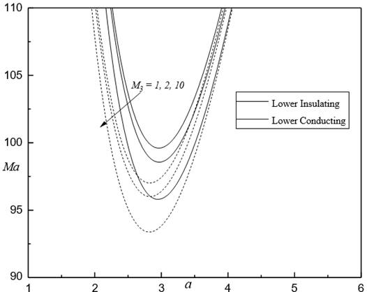
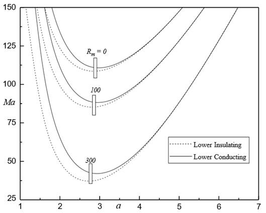
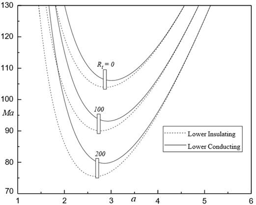
Figure 1,Figure 6 illustrates the
neutral stability curves corresponding for different ![]() ,
, ![]() ,
, ![]() ,
, ![]() ,
, ![]() and
and ![]() as well as different
bounding surfaces (surfaces of lower insulating and lower conducting). The
neutral stability curves are concave growing for each of these surfaces and the
curves of lower conducting case lie above lower insulating surfaces. The
neutral stability curves shift growing with
increasing Bi Figure 2, d Figure 3 representing that their
result is to increase
the stability region. Besides,
decrease the stability
of the region by increasing Ns Figure 4, M 3 Figure 5 Rm Figure 6 and Rt Figure 7
as well as different
bounding surfaces (surfaces of lower insulating and lower conducting). The
neutral stability curves are concave growing for each of these surfaces and the
curves of lower conducting case lie above lower insulating surfaces. The
neutral stability curves shift growing with
increasing Bi Figure 2, d Figure 3 representing that their
result is to increase
the stability region. Besides,
decrease the stability
of the region by increasing Ns Figure 4, M 3 Figure 5 Rm Figure 6 and Rt Figure 7
|
|
|
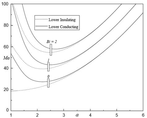
Figure 1 Ma against a for
R1= Rm =50, NS=5,
d = 0.5and M3 = 1 |
|
|
|
Figure 2 Ma against a for Rt = Rm
= 50 Ns = Bi = 5 and M3 = 1 |
|
|
|
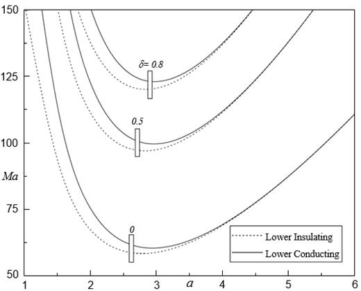
Figure 3 Ma against a for Rt = Rm
= 50, Bi = 5, d = 0.5 and M3 = 1 |
|
|
|
|
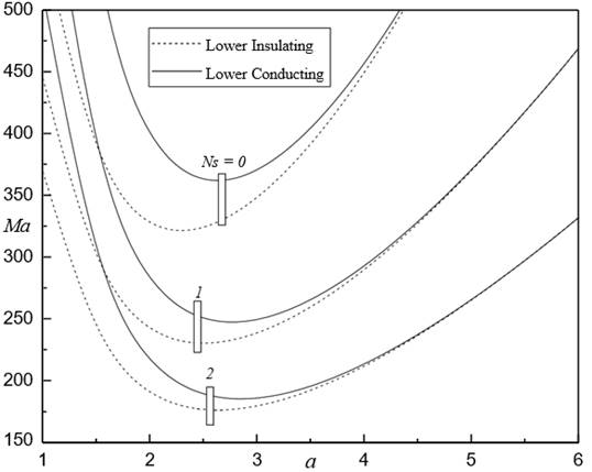
Figure 4 Ma against a for Rt = Rm
= 50, Bi = 5, d = 0.5 and Ns = 5 |
|
|
|
|
|
Figure 5 Ma against a for Rt
50, Bi = Ns = 5, d = 0.5 and M3 = 1 |
|
|
|
|
Figure 6 Ma against a for Rm = 50, Bi = Ns = 5, d = 0.5 and M3 = 1 |
|
|
|
Figure 7Mac against Bi
for different Rt when Rm = 50, Ns = 5, d = 0.5 and M3 = 1 |
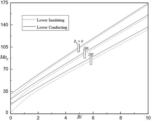
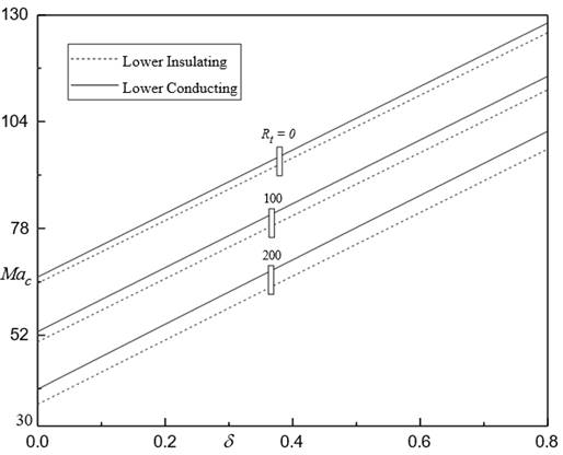
In Figure 8,Figure 11 analogous to solid
curves are corresponding to lower conducting and dotted curves corresponding to
lower insulating. The plot of ![]() against
against ![]() for various
for various ![]() for
for ![]()
![]() ,
, ![]() and
and ![]() Figure 7 It shows that the
Figure 7 It shows that the ![]() value of lower conducting and lower insulating by increasing
in
value of lower conducting and lower insulating by increasing
in ![]() . Clearly, the
results of lower insulating case are advancing the FTC compared to lower
conducting. A further reveal that an increase in
. Clearly, the
results of lower insulating case are advancing the FTC compared to lower
conducting. A further reveal that an increase in ![]() is to delay the onset
of FTC. This may be owing to the fact that with an increase in
is to delay the onset
of FTC. This may be owing to the fact that with an increase in![]() , the boundary of free surface departs from good conductor of
heat and hence there is an increase in Mac.
, the boundary of free surface departs from good conductor of
heat and hence there is an increase in Mac.
The effect of MFD viscosity parameter ![]() on the onset of FTC in a FF layer is presented in Figure 9 for fixed
on the onset of FTC in a FF layer is presented in Figure 9 for fixed ![]()
![]() ,
, ![]() and
and ![]() . It is viewed that
. It is viewed that ![]() increases with
increasing
increases with
increasing ![]() indicating its effect
is to stabilize the system. That is, the effect of
indicating its effect
is to stabilize the system. That is, the effect of ![]() increasing is to delay
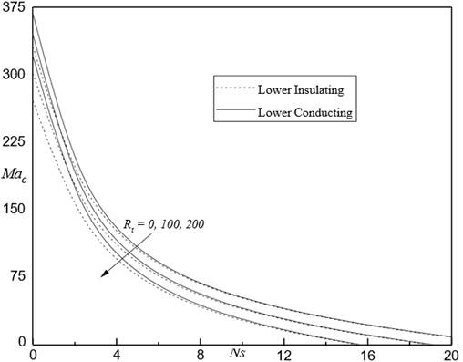
the FTC in the existence of magnetic field. To explore the effect of strength
of dimensionless internal heat source
increasing is to delay
the FTC in the existence of magnetic field. To explore the effect of strength
of dimensionless internal heat source ![]() on the measure for the
onset of FTC, the variation of
on the measure for the
onset of FTC, the variation of ![]() is displayed
against
is displayed
against ![]() for
for ![]()
![]() ,
, ![]() and
and ![]() . in Figure 9. It is seen that
. in Figure 9. It is seen that
![]() decreases quite hastily
first and then quite gradually monotonically with
decreases quite hastily
first and then quite gradually monotonically with ![]() representing the influence of increasing
internal heating is to decrease
representing the influence of increasing
internal heating is to decrease ![]() and thus destabilize
the system. In particular, it is seen that
the curves of
and thus destabilize
the system. In particular, it is seen that
the curves of ![]() coalesce for various physical parameters as the strength of internal heating
coalesce for various physical parameters as the strength of internal heating ![]() is increased.
is increased.
|
|
|
Figure 8 Mac against d for different Rt when Rm = 50 Ns = 5 Bi = 5 and M3 = 1 |
|
|
|
Figure 9 Mac against Ns
for different Rt when Rm = 50, d = 0.5, Bi = 5 and M3 = 1 |
|
|
|
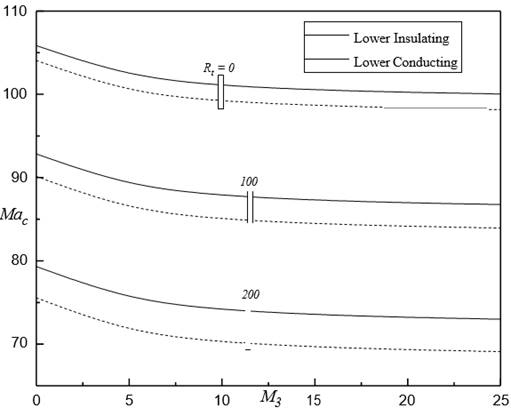
Figure 10 Mac
against M 3 for different Rt when
Rm = 50 Ns = 5 Bi = 5 and d = 0.5 |
|
|
|
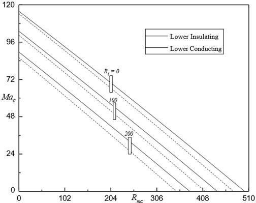
Figure 11 Mac
against Rmc for different Rt when M3 = 1 Ns = 5 Bi = 5 and d = 0.5 |
The
effect of increase in nonlinearity of fluid magnetization (i.e. M3 ) is shown in Figure 10 for different ![]() when
when![]()
![]() ,
, ![]() and
and ![]() . From the figure, it is seen that an increase in M3 is to decrease
. From the figure, it is seen that an increase in M3 is to decrease ![]() and thus increase in
the magnetization has destabilizing effects on the system but this effect is
very insignificant.
and thus increase in
the magnetization has destabilizing effects on the system but this effect is
very insignificant.
The locus plot of ![]() against for various
against for various ![]() for
for ![]()
![]() ,
, ![]() and
and ![]() Figure 11. It shows that they are bridging the space
between lower insulating and conducting cases by increasing in
Figure 11. It shows that they are bridging the space
between lower insulating and conducting cases by increasing in ![]() . For
. For ![]() , the case corresponds to only the surface tension force are
in effect. The amount of
, the case corresponds to only the surface tension force are
in effect. The amount of ![]() is associated to the importance of buoyancy gravitational
force. It is observed that increase in
is associated to the importance of buoyancy gravitational
force. It is observed that increase in ![]() leads to decrease
leads to decrease ![]() and
and ![]() signifying that the FF carries more heat efficiency than the
ordinary viscous fluid case. This due to an increase the destabilizing the
coupled magnetic and surface tension forces with increasing buoyancy
gravitational force,
signifying that the FF carries more heat efficiency than the
ordinary viscous fluid case. This due to an increase the destabilizing the
coupled magnetic and surface tension forces with increasing buoyancy
gravitational force, ![]() , thus the more easily for fluid flow in the system.
, thus the more easily for fluid flow in the system.
5. CONCLUSIONS
The linear stability theory is applied to study the
effect of MFD viscosity on coupled buoyancy-gravitational and surface-tension
forces on FTC in a FF layer through the strength of internal heat source on the
system under the conditions of lower insulating/conducting case. The FF layer is heated from below and its top
surface is subjected to a surface-tension force decreasing linearly with
temperature. The problem of resulting eigenvalue is obtained numerically by
utilizing the Galerkin WRT technique. It is shown that the effect of MFD
viscosity is to enhance the onset of FTC and hence MFD viscosity plays a
stabilizing role on the system. The increase in buoyancy-gravitational force,
the forces of magnetic and surface-tension effect is to destabilize the system.
Their effects are complementary in the sense that the critical ![]() and
and ![]() decrease with an increase in
decrease with an increase in ![]() . The increase in
. The increase in ![]() ,
, ![]() and decrease in
and decrease in ![]() , M3 are
having stabilizing effect on the system.
, M3 are
having stabilizing effect on the system.
ACKNOWLEDGEMENTS
The authors (CEN) and (MKR) wish to thank the Management and Principal of Dr. Ambedkar Institute of Technology, and MES Pre-University College of Arts, Commerce and Science, Bangalore, respectively, for their encouragement.
REFERENCES
Blums, E. (2002). Heat And Mass Transfer Phenomena. https://link.springer.com/chapter/10.1007/3-540-45646-5_7
Blythe, P. A. And Simpkins, P. G. (1981). Convection In A Porous Layer For A Temperature Dependent Viscosity", International Journal Of Heat And Mass Transfer,24(3), 497-506. https://doi.org/10.1016/0017-9310(81)90057-0
Charles, S. W. (2002). The Preparation Of Magnetic Fluids. https://doi.org/10.1007/3-540-45646-5_1
Kassoy D. R. And Zebib, A. (1975). Variable Viscosity Effects On The Onset Of Convection In Porous Media", 18(12), 1649-1651. https://doi.org/10.1063/1.861083
Lebon, G. And Cloot, A. (1986). A Thermodynamical Modeling Of Fluid Flows Through Porous Media", Application Kassoy Dr, Zebib A. Variable Viscosity Effects On The Onset Of Convection In Porous Media To Natural Convection, International Journal Of Heat And Mass Transfer, 29(3), 381-389. https://doi.org/10.1016/0017-9310(86)90208-5
Nanjundappa, C. E. Ravisha, M. Lee, J. And Shivakumara, I. S. (2011). Penetrative Ferroconvection In A Porous Layer”, 243-257. https://doi.org/10.1007/s00707-010-0367-9
Nanjundappa, C. E. Shivakumara, I. S, And Prakash, H. N. (2012). Penetrative Ferroconvection Via Internal Heating In A Saturated Porous Layer With Constant Heat Flux At The Lower Boundary", Journal Of Magnetism Magnetic Materials, 324(9), 1670-1678. https://doi.org/10.1016/j.jmmm.2011.11.057
Nanjundappa, C. E. Shivakumara, I. S. Lee, J. And Ravisha, M. (2011). Effect Of Internal Heat Generation On The Onset Of Brinkman-Bénard Convection In A Ferrofluid Saturated Porous Layer", International Journal Of Thermal Sciences, 50(2), 160-168. https://doi.org/10.1016/j.ijthermalsci.2010.10.003
Nield, D. A. (1964). Surface Tension And Buoyancy Effects In Cellular Convection, Journal Of Fluid Mechanics, 19(3), 341-352. https://doi.org/10.1017/S0022112064000763
Nkurikiyimfura, I. Wanga, Y. And Pan, Z. (2013). Heat Transfer Enhancement By Magnetic Nanofluids-A Review", Renewable And Sustainable Energy Reviews, 548-561. https://doi.org/10.1016/j.rser.2012.12.039
Patil, P. R. And Vaidyanathan, G. (1981). Effect Of Variable Viscosity On The Setting Up Of Convection Currents In A Porous Medium", International Journal Of Engineering Sciences, 421-426. https://doi.org/10.1016/0020-7225(81)90062-8
Patil, P. R. And Vaidyanathan, G. (1982). Effect Of Variable Viscosity On Thermohaline Convection In A Porous Medium", Journal Of Hydrology, 147-161. https://doi.org/10.1016/0022-1694(82)90109-3
Rosensweig, R. E. (1985). Ferrohydrodynamics, https://www.cambridge.org/core/journals/journal-of-fluid-mechanics/article/abs/ferrohydrodynamics-by-r-e-rosensweig-cambridge-university-press-1985-344-pp-45/F9ED8D5FBD40AD7CFF5CB1D827ADA3CC
Rosenwieg, R.E. Kaiser, R. Miskolczy, G. (1969). Viscosity Of Magnetic Fluid In A Magnetic Field" Journal Of Colloid Interface Science, 680-686. https://doi.org/10.1016/0021-9797(69)90220-3
Savitha, Y. L. Nanjundappa, C. E. And Shivakumara, I. S. (2021). Penetrative Brinkman Ferroconvection Via Internal Heating In High Porosity Anisotropic Porous Layer : Influence Of Boundaries", https://doi.org/10.1016/j.heliyon.2021.e06153
Shivakumara, I. S. Lee, J. And Nanjundappa, C. E. (2012). Onset Of Thermogravitational Convection In A Ferrofluid Layer With Temperature Dependent Viscosity", Asme Journal Of Heat Transfer, 134(1). https://doi.org/10.1115/1.4004758
Shliomis, M. L. (1974). Magnetic Fluids", 17(2), 153. https://doi.org/10.1070/PU1974v017n02ABEH004332
Sparrow, E. W. Goldstein, R. J. And Jonson, V. K. (1964). Thermal Instability In A Horizontal Fluid Layer : Effect of Boundary Conditions And Nonlinear Temperature Profile", Journal of Fluid Mechanics, 513-528. https://doi.org/10.1017/S0022112064000386
Vaidyanathan, G. Sekar, R. Ramanathan, A. (2002). Effect of Magnetic Field Dependent Viscosity On Ferroconvection In Rotating Porous Mediu, Indian Journal of Pure And Applied Mathematics, 159-165. https://doi.org/10.1016/S0304-8853(02)00355-4
|
|
 This work is licensed under a: Creative Commons Attribution 4.0 International License
© IJETMR 2014-2022. All Rights Reserved.