Mathematical Strategies for Solving Optimization Problems

 

Dr. Yogeesh N ¹ , Girish Yadav K. P ², Dr. Girija D.K ³ , N. Raja ⁴

 

¹ Assistant Professor, Department of Mathematics, Government First Grade College, Tumkur, Karnataka, India

² Assistant Professor, Department of Mathematics, Vedavathi Government First Grade College, Hiriyur, India

³ Associate Professor and HOD, Department of Computer Science, Government First Grade College, Madhugiri, Karnataka, India

⁴ Assistant Professor, Department of Visual Communication, Sathyabama Institute of Science and Technology, Deemed University, A++ Grade by NAAC & Category 1 University by UGC, Chennai, Tamilnadu, India

 

1. INTRODUCTION

A collection of mathematical concepts and methods are employed in the subject of optimisation, also known as mathematical programming, to address quantitative issues in a variety of disciplines, including engineering, the physical sciences, business, statistical economics, and the biological sciences. This subject emerged from the understanding that quantitative issues in seemingly disparate disciplines share significant mathematical aspects, and taking advantage of these similarities, many more problems can be defined and solved using the various procedures and techniques that constitute the study of optimization theory [1].

Mathematical programming, which is mainly synonymous with optimization, was derived in 1940 [2]. Before that, the term programming was associated with computer programming and became synonymous with it. Research into the mathematical formulation of optimal problems, the creation of various approaches for doing so, the mathematical investigation of various characteristics displayed by those approaches, and the application of such approaches on computers are some of the topics covered by mathematical programming [3]. The complex nature of optimization problems that can be solved has increased dramatically as a result of faster computers. Optimization problems can be found in the subject of mathematics, computational science, and statistical economics to obtain the optimal solutions from all feasible options. Depending on their nature, optimization has two types: continuous and discrete optimization problems.

Discrete optimisation deals with optimisation issues using discrete variables, where a countable collection of factors must be used to identify an object such as an integer, permutation, or graph [4]. On the other hand, issues involving continuous optimisation must be solved in order to determine the optimal value from a continuous function. These problems can involve challenges with constraints as well as problems with many modes of transportation [5].

The programme generates an optimisation issue that has to be addressed while doing parameter estimation. The estimated model parameter set is an example of an optimisation problem's solution. The variables, restrictions, and objective functions that make up this optimisation problem are listed below [6].

1)    Design of variable:

Estimating the model's parameters and initial states is required.

2)    Objective of the functions:

This is a function that generates a measure of how much the calculated responses differ. Cost function and estimation error are other terms for the same thing.

3)    Bound Values:

Limits on the predicted parameter values have been established.

4)    Constraint-functions:

A function which specifies limits on the variables used in a process of design.

The optimizing solver adjusts the value of a design parameters in order-to meet the objectives & constraints that have been stated. According to the optimization approach that we employ to get precise solution for various problems of optimization.

Now, the situation of unconstrained optimum, the necessary & sufficient criteria for a local minimum may result in a system of equations which are too hard to solve analytically, similar to the event of unconstrained optimization. Indeed, the presence of constraints makes the problem far more difficult to solve much faster! As a result, we must once again rely on numerical algorithms, which, in the case of the equality-constrained problems, will be built by altering the "steepest-descent" processes that were previously described.

 

2. OPTIMIZATION TECHNIQUES AND ISSUES

Optimization problems will be divided into the following classifications:

 

1)    Minimization-problems

A function f(x) is an objective function that is minimised. It is necessary to specify the frequency representation that you wish the final model to follow. Optionally, you can define upper and lower boundaries for the estimated coefficients.

2)    Mixed minimization and feasible problems

 A minimization problem is one that minimises an objective functions f(x), within defined limitations and constraints, C(x). As well as specifying the measured signal because you want its model to track, you can define bounds and restrictions for the predicted values as well as the estimated parameters.

3)    Feasibility-problems

 Finding a solution that meets the provided restrictions, C(x) is performed. You only define bounds and limitations for the predicted values in this section. In the field of parameter estimation, this type of difficulty is uncommon.

 

3. TECHNIQUES FOR OPTIMIZATION OF VARIOUS TYPES

The classification of the optimization model is a critical phase in the optimization technique because the algorithms used to solve optimization problems are adapted upon type of issues under consideration. Consider the following examples of different optimization problem types:

1)    Continuous Optimization vs. Discrete Optimization is a comparison of two types of optimizations.

In contrast to models with discrete variables, models having continuous variables were discrete optimization issues, whereas models with discrete variables can be continuous optimization problems Continuous optimization problem is less difficult to get solution that discrete optimal issues, and hence are more common. An integer, permutations, or graph are examples of objects that can be found in a countable set when solving a discrete optimization model, which is defined as follows: As a result of improvements in algorithms, combined with advancements in cognitive computing, the size-complexity for discrete algorithms of optimization those will be addressed efficiently have grown in both size and complexity. The importance of continuous optimization methods in discrete optimization cannot be overstated, as many discrete optimization procedures create a succession of continuous sub-problems.

2)    Optimization with no constraints versus Optimization with constraints

The difference between issues where there are constraints upon this variable and limitations in which there are no constraints upon that variables is a critical distinction among optimization problems and other types of problems.

It is common for unconstrained optimization issues to occur in many actual applications, but they can also arise as a result of the reformulation existing constrained optimization problems. Constrained optimization difficulties arise in situations where the variables are subjected to explicit limits on their behavior. Constrained optimization techniques are further subdivided based on the nature of the constraints, such as nonlinear, convex, linear and function smoothness, including such differentiable or non-differentiable, as well as the type of optimization problem.

 

3)    Objectives can be one, several, or none at all

Despite the fact that the vast majority of optimization problems get a single objective function, there have been several unusual examples in which optimization problem have either no objective function or many objective functions. Multi-objective optimization problems emerge in a various type of subjects, including engineering-technology, statistical economics, and concept of logistics, among others. Frequently, problems along various aims are reformed as problems of single objectivity to simplify their complexity.

4)    What is the difference between Deterministic Optimization and Stochastic Optimization?

It is possible to perform deterministic optimization when all of the data for a given problem is known with certainty. However, for a variety of reasons, it is not always possible to obtain precise information on the data. A simple measurement error could be the source of the problem. The fact that some facts contain data and facts means that they can be known with certainty for another reason. When uncertainty is integrated into a model in the context of optimization under uncertainty, the process is referred to as stochastic optimization.

 

4. GENERALLY SPEAKING, OPTIMIZATION PROBLEM WILL BE OF TWO VARIETIES

1)    Linear-Programming

The linear-programming (LP) problems, will have the objective of linear (continuous) functions of decision variables with their constraints. The fact that all linear methods are convex means that solving general linear problem is inherently easier than solving non-linear problems in most cases.

Simple techniques for finding the best conclusion, or more accurately optimum points of complex relationships expressed by linear relationships are available. Linear programming is one of these techniques. Simpler terms: the real-world interactions could be far more complex, but they can be reduced to linear relationships by simplifying them.

Linear programming is commonly utilised in optimization for a variety of reasons, some of which are as follows:

In operation research, complicated real-world problems will be defined as linear-programming problems, which can be applied to various situations.

Many algorithms in certain types of optimization issues operate by treating Linear Programming problem as sub-problems, which is a common practice in the optimization community.

Most fundamental notions in optimization theory, including duality, decomposition, convexities, and convexity generalisations, were inspired by it and derived from ideas in linear programming.

Linear-programming were utilised in the beginning stages of the development of micro-economics, and now it is being used today in the areas such as plan-production-transport, and technology, among others.

·        Expressing Linear optimization problems as LPP

The Linear Programming Problems (LPP), often known as the linear optimization problem, is a type of optimization problem. If the criteria of a mathematical model are expressed by linear connections, then it is a method of achieving the best (optimal) result, such as the largest predicted portfolio returns risk level, by optimising the model. The following is the typical form for LPP:

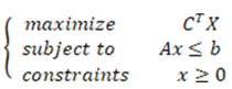                                                                                                        (1)

 

In (1), Where   is our objective function, is a constraints group, and will be another constraints group. We can use a variety of different forms to meet the requirements.

·        Example Problem involving optimization

A collection of constraint that is defined using following set of line equations.

 

                                                                                         (2) 

 

The boundaries of given points including endless set of all the points which represents feasible set of solutions from (2).

Figure 1

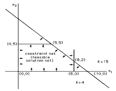
Figure 1 Graph Showing Feasible Solutions

 

2)    Quadratic Programming

The objective function of a decision variables is a complex quantity of the variable, and the all constraints are linear-function of every decision-variables as in quadratic programming problems.

Example of a Quadratic-Programming issue that is extensively utilised is the Markowitz average portfolio optimization technique, where the objectives are to minimise portfolio variance while the linear constraints mandate a lower bound on portfolio return.

Quadratic programming is a method for solving a special kind of optimization issue in which it optimises (minimises or maximises) the objectives of quadratic functions with respect to one or many linear-constraints. It is also called as quadratic programming. Non-linear programming is another name for quadratic programming, which is sometimes used to refer to it.

In QP, the objective function may contain bilinear terms or polynomial terms of up to second order. Constraints are typically linear in nature, and they can include both equality and inequality.

Quadratic Programming is a technique that is commonly employed in optimization. The following are the reasons: The following are the reasons:

·        Portfolio optimization is a term used to describe the optimizing of financial portfolios.

·        Using the least-squares regression method to analyse data.

·        Scheduling control in chemical plants is important.

·        Using non-linear programming to solve more sophisticated non-linear programming problems.

·        The application of statistics in operations research & statistical work

 

5. QUADRATIC OPTIMIZATION PROBLEMS

It is proposed that we study the following two types of quadratic optimization issues that are commonly encountered both in the field of engineering or in subject computer science (particularly in computational concepts):

Minimization:  ,or with respect to affine or linear-constraints.

Minimization:    over the unit sphere.

A is a symmetric matrix in both of these instances. We are also looking for the circumstances that are required & more sufficient for f to provide a global-minimum. Many more issues of engineering & physics will be expressed as a minimizing of functions f, with/without constraints, and can be expressed in this manner. Natural processes are designed to reduce energy consumption, which is an important principle of mechanics. Additionally, if a physical model would be in a sustainable equilibrium, the energies stored within that condition must be at its lowest possible level (or zero). A quadratic function is the simplest type of energy function that may be defined.

The functions are defined in the form of, Here A is called symmetrical matrix of order , &  are vectors in the , viewed as a column-vectors.

Primal Quadratic Optimization Problems:

 

 

 

Dual-Quadratic Optimization Problems:

 

 

 

KKT Conditions

 

 

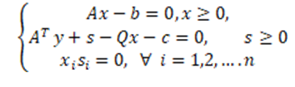
Where A is called symmetrical matrix of order, &   are vectors in the, viewed as a column-vectors and   is our objective function, is a constraints group, and will be another constraints group.

 

6. CHOICE OF OPTIMIZER

Now a days, the optimizer that is used has an impact on both the pace of convergence & whether or not it occurs. In recent years, a number of options to the traditional gradient descent algorithms, and these are mentioned in mathematical formulae according to requirement of the problem.

 

7. CASE STUDY: LINEAR PROGRAMMING FOR PRODUCTION OPTIMIZATION.

Let's look at a fictitious case study where a business manufactures two different product categories, A and B. The production process makes use of the two machines X as well as Y. In order to maximise profit, the company tries to determine the best production levels of each product within the constraints of the available resources and other considerations.

The manufacturing capacity, cost of production, and selling price of each product are displayed in the following table:

Table 1

Table 1 Comparision of Manufacturing Capacity, Cost of Production, and Selling Price of Each Product
Product	Production Capacity (units)	Production Cost (per unit)	Selling Price (per unit)
A	400	15	25
B	500	18	30

 

Figure 2

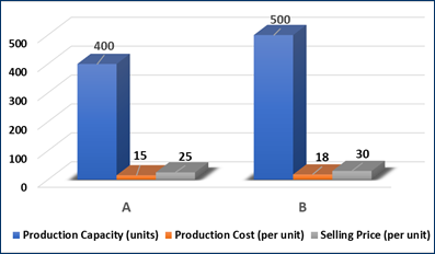
Figure 2 Graph Showing Manufacturing Capacity, Cost of Production, and Selling Price of Each Product

 

The production process involves two machines, X and Y, with the following production times and requirements:

Table 2

Table 2 Optimal Production Times and Requirements for Each Product
Machine	Production Time for A (hours per unit)	Production Time for B (hours per unit)	Available Hours per week
X	2	1	80
Y	1	2	60

 

The objective is to determine the optimal production levels for each product, subject to the available resources and constraints.

Solution: This is an illustration of a linear programming issue, where the goal is to maximise profit while taking into account linear restrictions.

Let's assume that the production levels of product A and B are represented by x and y, respectively. The objective function may thus be written as follows:

Maximize Profit = 25x + 30y - (15x + 18y)

Simplifying the expression, we get:

Maximize Profit = 10x + 12y

The constraints can be expressed as:

2x + y <= 80; x + 2y <= 60

x <= 400; y <= 500; x >= 0; y >= 0

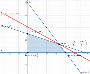
Figure 3

 

Table 3 Graph Showing Feasible Region of Optimal Solution

 

Here are the outcomes of the objective function for each of the places in the feasible zone shown in Figure 3 (in this graph, x and y are equal to X1 and X2, respectively).

Using the Simplex approach to solve the aforementioned issue, we arrive at the following ideal result:

x = 200, y = 200

The maximum profit that can be achieved is:

Profit = 10x + 12y = 10(200) + 12(200) = 4400

Therefore, the optimal production levels for products A and B are 200 units each, which will result in a maximum profit of $4400.

Summary of the case study: In this case study, we solved an optimisation problem using a mathematical strategy, more precisely linear programming. The optimal production levels for items A and B have been determined based on the available resources and constraints. This strategy may be used to solve a number of practical issues, including supply chain optimisation, resource allocation, and production planning.

 

8. SCOPE FOR FUTURE STUDY

Future research on optimising output levels using linear programming has a huge potential. Some possible study directions include:

1)    Creation of more intricate models: The case study in this work took into account a streamlined linear programming model. In order to more accurately represent the complexity of actual industrial operations, future research may investigate the use of more sophisticated models, such as mixed-integer linear programming.

2)    Integration with other optimisation techniques: To produce hybrid optimisation approaches, linear programming may be combined with other optimisation strategies like genetic algorithms or simulated annealing. Future research might examine how well these hybrid production level optimisation techniques work.

3)    Incorporation of uncertainty: Supply chain interruptions and fluctuating demand are two common sources of uncertainty that affect manufacturing operations. Future research may examine the application of stochastic programming to describe uncertainty in production optimisation.

4)    Application to different industries: Although the case study in this paper concentrated on a manufacturing firm, linear programming may be utilised to solve optimisation issues in a number of different businesses. The use of linear programming in industries including logistics, transportation, and finance might be explored in further research.

Overall, the application of linear programming in production optimisation is a promising field for future study, with lots of room for growth and improvement.

 

9. CONCLUSION

When it comes to the study of discretization principles, optimization theory can yield valuable insights regardless of whether a mathematical formulation to a particular situation is sought or not. The successful solutions of problems in this vein is typically based on a marriage between approaches in regular "continuous" optimization and particular ways of dealing with specific types of combinatorial structure in certain situations. The study of networks is one of the major fields in and that there have been significant accomplishments as well as interesting theoretical breakthroughs (directed graphs). In case of network flow and potentials, there are an astonishing number of problems that may be created and solved. Convex functions include all linear functions as well as some quadratic functions, as well as the conic constraints of conic-optimization problem, which were also a convex-functions. Some of the smooth curve non-linear functions are convexity, but not all of them are. Numerical and constraint programming issues, by their very nature, are non-convex. Global optimization techniques are useful to handle problems that are not convex in nature.

Remember that only the sections of your objectives and constraint formulations that depend on the choice variables count. This parallels breakthroughs in computer science, operations research, game theory, numeric analysis, control theory, combinatorics. and statistical/mathematical economics, Typical concept of optimization issues included three components. On can maximize or minimize a single numerical number, or objective function. Hence, this paper has helped us know the idea of Mathematical Approaches to Different Optimization Problems.

 

CONFLICT OF INTERESTS

None. 

 

ACKNOWLEDGMENTS

None.

 

REFERENCES

R. Fletcher, Practical Methods of Optimization, John Wiley & Sons, 2013.

D. P. Bertsekas, Nonlinear Programming, Athena Scientific, 2016.

S. Boyd and L. Vandenberghe, Convex Optimization, Cambridge University Press, 2004.

A. Charnes and W. W. Cooper, Management Models and Industrial Applications of Linear Programming, Vol. 1, Wiley-Interscience, 1961.

J. Nocedal and S. Wright, Numerical Optimization, Springer, 2006.

M. Biegler, Nonlinear Programming: Concepts, Algorithms, and Applications to Chemical Processes, SIAM, 2010.

Auger A., Teytaud O. (2010) Continuous lunches are free plus the design of optimal optimization algorithms. Algorithmica, 57, 121–146.

Yogeesh N. "Study on Clustering Method Based on K-Means Algorithm." Journal of Advances and Scholarly Researches in Allied Education (JASRAE), vol. 17, no. 1, 2020, pp. 485-489(5), www.ignited.in//I/a/305304.

Dennis J.E.Jr. et al.  (1981) An adaptive nonlinear least-squares algorithm. ACM Trans. Math. Softw. (TOMS), 7, 348–368.

Egea J.A. et al.  (2009) Dynamic optimization of nonlinear processes with an enhanced scatter search method. Ind. Eng. Chem. Res., 48, 4388–4401.

Yogeesh N. "Mathematical Approach to Representation of Locations Using K-Means Clustering Algorithm." International Journal of Mathematics And its Applications (IJMAA), vol. 9, no. 1, 2021, pp. 127-136.

Esposito W.R., Floudas C. (2000) Global optimization for the parameter estimation of differential-algebraic systems. Ind. Eng. Chem. Res., 39, 1291–1310.

Hendrix E., Tóth B. (2010) Introduction to Nonlinear and Global Optimization. Springer Verlag, New York.

Hindmarsh A.C. et al.  (2005) Sundials: suite of nonlinear and differential/algebraic equation solvers. ACM Trans. Math. Softw. (TOMS), 31, 363–396.